Online Tutorial on Regression Modeling with Actuarial and Financial Applications
Preface
Date: 01 October 2024
About Regression Modeling
Statistical techniques can be used to address new situations. This is important in a rapidly evolving risk management world. Analysts with a strong analytical background understand that a large data set can represent a treasure trove of information to be mined and can yield a strong competitive advantage. This book and online tutorial provides budding analysts with a foundation in multiple reression. Viewers will learn about these statistical techniques using data on the demand for insurance, healthcare expenditures, and other applications. Although no specific knowledge of actuarial or risk management is presumed, the approach introduces applications in which statistical techniques can be used to analyze real data of interest.
Resources
- This tutorial is based on the book Regression Modeling with Actuarial and Financial Applications.
- For resources associated with the book, please visit the Regression Modeling book web site.
- For advanced regression applications in insurance, you may be interested in the series, Predictive Modeling Applications in Actuarial Science.
- Sample code and data for the series are available at series website.
- An earlier version of this tutorial, a Short Course constructed for Indonesian actuaries, uses the Datacamp learning platform.
Tutorial Description
- This online tutorial is designed to guide you through the foundations of regession with applications in actuarial science.
- Anticipated completion time is approximately six hours.
- The tutorial assumes that you are familiar with the foundations in the statistical software
R, such as Datacamp’s Introduction to R.
General Layout. There are five chapters in this tutorial that summarize the foundations of multiple linear regression. Each chapter is subdivided into several sections. At the beginning of each section is a short video, typically 4-8 minutes, that summarizes the section key learning outcomes. Following the video, you can see more details about the underlying R code for the analysis presented in the video.
Role of Exercises. Following each video, there are one or two exercises that allow you to practice skills to make sure that you fully grasp the learning outcomes. The exercises are implented using an online learning platfor provided by Datacamp so that you need not install R. Feedback is programmed into the exercises so that you will learn a lot by making mistakes! You will be pacing yourself, so always feel free to reveal the answers by hitting the Solution tab. Remember, going through quickly is not equivalent to learning deeply. Use this tool to enhance your understanding of one of the foundations of data science, regression analysis.
Aquí está el Prefacio en español
Welcome to the Tutorial Video
In this video, you learn how to:
- Describe regression briefly, i.e., in a nutshell
- Explain Galton’s height example as a regression application
En Español
Video Overhead
A. Galton’s 1885 Regression Data
\[ \small{\begin{array}{l|ccccccccccc|c} \hline \text{Height of }& & & & & & & & & & & & \\ \text{adult child }& & & & & & & & & & & & \\ \text{in inches }& <64.0 & 64.5 & 65.5 & 66.5 & 67.5 & 68.5 & 69.5 & 70.5 & 71.5 & 72.5 & >73.0 & \text{Totals} \\ \hline >73.7 & - & - & - & - & - & - & 5 & 3 & 2 & 4 & - & 14 \\ 73.2 & - & - & - & - & - & 3 & 4 & 3 & 2 & 2 & 3 & 17 \\ 72.2 & - & - & 1 & - & 4 & 4 & 11 & 4 & 9 & 7 & 1 & 41 \\ 71.2 & - & - & 2 & - & 11 & 18 & 20 & 7 & 4 & 2 & - & 64 \\ 70.2 & - & - & 5 & 4 & 19 & 21 & 25 & 14 & 10 & 1 & - & 99 \\ 69.2 & 1 & 2 & 7 & 13 & 38 & 48 & 33 & 18 & 5 & 2 & - & 167 \\ 68.2 & 1 & - & 7 & 14 & 28 & 34 & 20 & 12 & 3 & 1 & - & 120 \\ 67.2 & 2 & 5 & 11 & 17 & 38 & 31 & 27 & 3 & 4 & - & - & 138 \\ 66.2 & 2 & 5 & 11 & 17 & 36 & 25 & 17 & 1 & 3 & - & - & 117 \\ 65.2 & 1 & 1 & 7 & 2 & 15 & 16 & 4 & 1 & 1 & - & - & 48 \\ 64.2 & 4 & 4 & 5 & 5 & 14 & 11 & 16 & - & - & - & - & 59 \\ 63.2 & 2 & 4 & 9 & 3 & 5 & 7 & 1 & 1 & - & - & - & 32 \\ 62.2 & - & 1 & - & 3 & 3 & - & - & - & - & - & - & 7 \\ <61.2 & 1 & 1 & 1 & - & - & 1 & - & 1 & - & - & - & 5 \\ \hline \text{Totals }& 14 & 23 & 66 & 78 & 211 & 219 & 183 & 68 & 43 & 19 & 4 & 928 \\ \hline \end{array}} \]
B. Supporting R Code
# Reformat Data Set
#heights <- read.csv("CSVData\\GaltonFamily.csv",header = TRUE)
heights <- read.csv("https://assets.datacamp.com/production/repositories/2610/datasets/c85ede6c205d22049e766bd08956b225c576255b/galton_height.csv", header = TRUE)
str(heights)
head(heights)
heights$child_ht <- heights$CHILDC
heights$parent_ht <- heights$PARENTC
heights2 <- heights[c("child_ht","parent_ht")]
#heights <- read.csv("CSVData\\galton_height.csv",header = TRUE)
heights <- read.csv("https://assets.datacamp.com/production/repositories/2610/datasets/c85ede6c205d22049e766bd08956b225c576255b/galton_height.csv", header = TRUE)
plot(jitter(heights$parent_ht),jitter(heights$child_ht), ylim = c(60,80), xlim = c(60,80),
ylab = "height of child", xlab = "height of parents")
abline(lm(heights$child_ht~heights$parent_ht))
abline(0,1,col = "red", lty=2)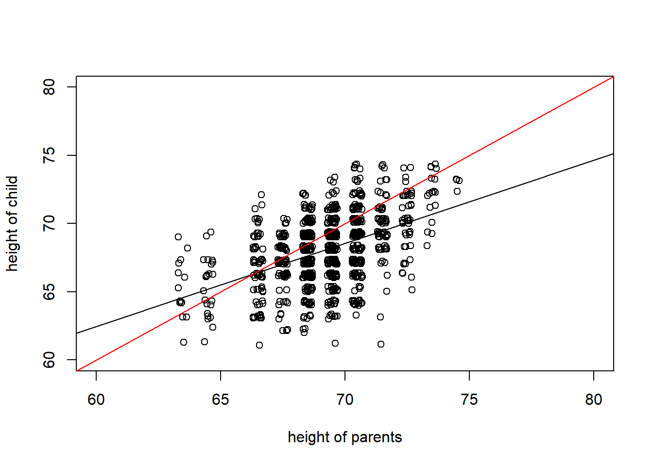
Call:
lm(formula = heights$child_ht ~ heights$parent_ht)

Residuals:
    Min      1Q  Median      3Q     Max
-8.2577 -1.4280  0.1323  1.5720  5.7918

Coefficients:
                  Estimate Std. Error t value Pr(>|t|)
(Intercept)       25.84856    2.69009   9.609   <2e-16 ***
heights$parent_ht  0.60992    0.03882  15.710   <2e-16 ***
---
Signif. codes:  0 '***' 0.001 '**' 0.01 '*' 0.05 '.' 0.1 ' ' 1

Residual standard error: 2.26 on 926 degrees of freedom
Multiple R-squared:  0.2104,    Adjusted R-squared:  0.2096
F-statistic: 246.8 on 1 and 926 DF,  p-value: < 2.2e-16