Chapter 2 Basic Linear Regression

Chapter description

This chapter considers regression in the case of only one explanatory variable. Despite this seeming simplicity, many deep ideas of regression can be developed in this framework. By limiting ourselves to the one variable case, we can illustrate the relationships between two variables graphically. Graphical tools prove to be important for developing a link between the data and a predictive model.

2.1 Correlation

In this section, you learn how to:

Calculate and interpret a correlation coefficient
Interpret correlation coefficients by visualizing scatter plots

2.1.1 Video

Video Overhead Details

A Details. Wisconsin lottery data description

Lot <- read.csv("CSVData\\Wisc_lottery.csv")
#Lot <- read.csv("https://assets.datacamp.com/production/repositories/2610/datasets/a792b30fb32b0896dd6894501cbab32b5d48df51/Wisc_lottery.csv", header = TRUE)
str(Lot)

'data.frame':   50 obs. of  3 variables:
 $ pop    : int  435 4823 2469 2051 13337 17004 38283 9859 4464 20958 ...
 $ sales  : num  1285 3571 2407 1224 15046 ...
 $ medhome: num  71.3 98 58.7 65.7 96.7 66.4 91 61 91.5 68.8 ...

B Details. Summary statistics

#options(scipen = 100, digits = 4)
#numSummary(Lot[,c("pop", "sales")], statistics = c("mean", "sd", "quantiles"), quantiles = c(0,.5,1))
(as.data.frame(psych::describe(Lot)))[,c(2,3,4,5,8,9)]
#Rcmdr::numSummary(Lot[,c("pop", "sales")], statistics = c("mean", "sd", "quantiles"), quantiles = c(0,.5,1))

         n     mean          sd   median   min     max
pop     50 9311.040 11098.15695 4405.500 280.0 39098.0
sales   50 6494.829  8103.01250 2426.406 189.0 33181.4
medhome 50   57.092    18.37312   53.900  34.5   120.0

C Details. Visualizing skewed distributions

par(mfrow = c(1, 2))
hist(Lot$pop, main = "", xlab = "population")
hist(Lot$sales, main = "", xlab = "sales")

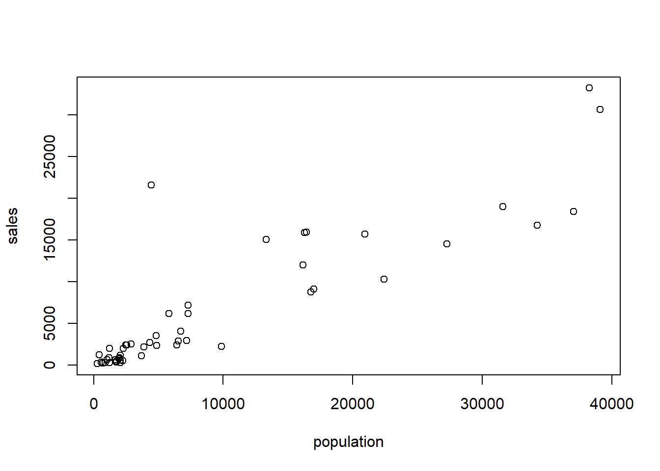
D Details. Visualizing relationships with a scatter plot

plot(Lot$pop, Lot$sales, xlab = "population", ylab = "sales")

E Details. Correlation coefficient

cor(Lot$pop, Lot$sales)

[1] 0.8862827

2.1.2 Exercise. Correlations and the Wisconsin lottery

Assignment Text

The Wisconsin lottery dataset, Wisc_lottery,has already been read into a dataframe Lot.

Like insurance, lotteries are uncertain events and so the skills to work with and interpret lottery data are readily applicable to insurance. It is common to report sales and population in thousands of units, so this exercise gives you practice in rescaling data via linear transformations.

Instructions

From the available population and sales variables, create new variables in the dataframe Lot, pop_1000 and sales_1000 that are in thousands (of people and of dollars, respectively).
Create summary statistics for the dataframe that includes these new variables.
Plot pop_1000 versus sales_1000.
Calculate the correlation between pop_1000 versus sales_1000 using the function cor(). How does this differ between the correlation between population and sales in the original units?

2.2 Method of least squares

In this section, you learn how to:

Fit a line to data using the method of least squares
Predict an observation using a least squares fitted line

2.2.1 Video

2.2.1.1 Video Overheads

A Details. Where to fit the line?

model_blr <- lm(sales ~ pop, data = Lot)
plot(Lot$pop, Lot$sales,xlab = "population", ylab = "sales")
abline(model_blr, col="blue")
abline(0,1, col="red")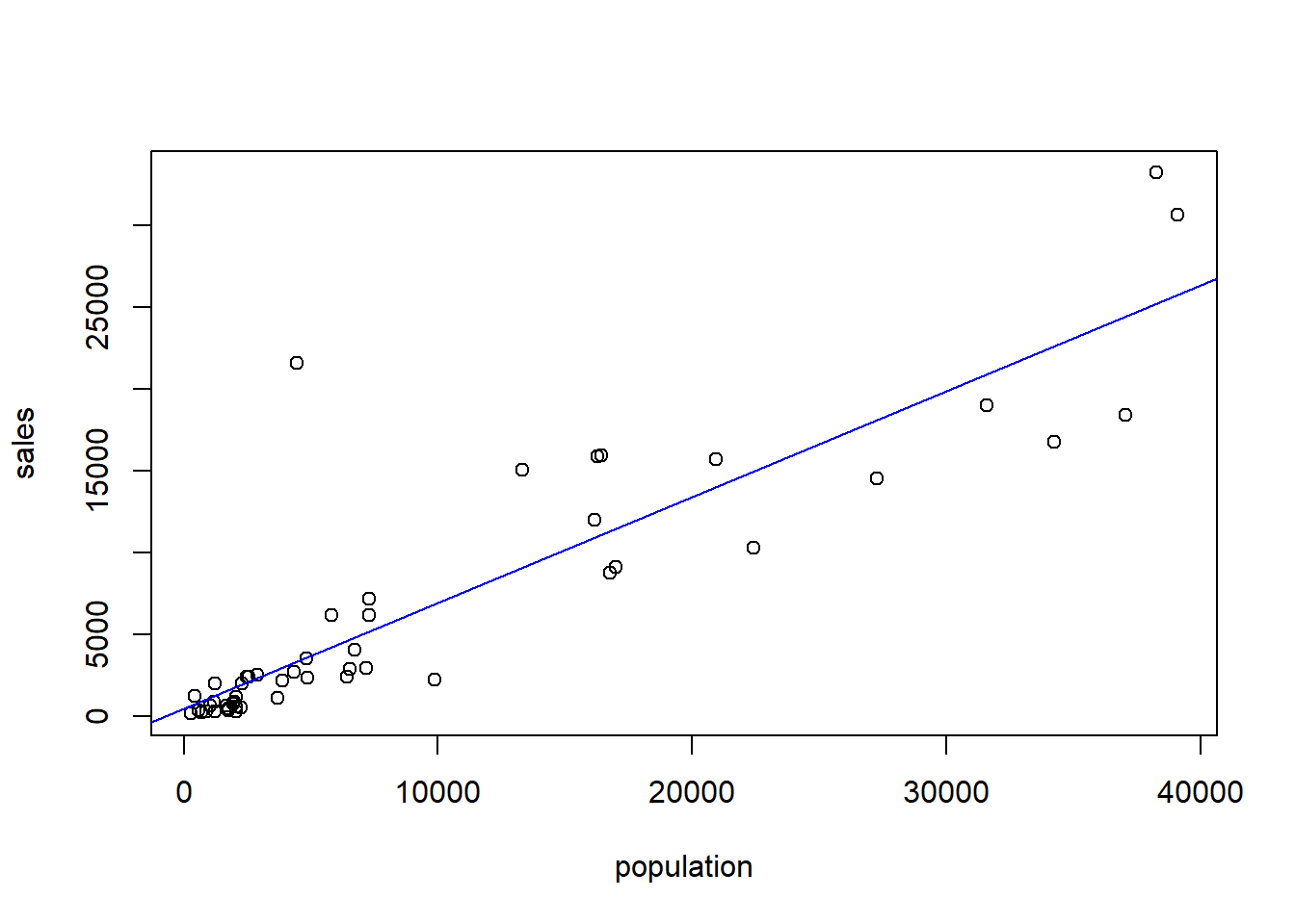

B Details. Method of least squares

For observation $\{(y, x)\}$, the height of the regression line is \[b_0 + b_1 x.\]
Thus, $y - (b_0 + b_1 x)$ represents the deviation.
The sum of squared deviations is \[SS(b_0, b_1) = \sum (y - (b_0 + b_1 x))^2 .\]
The method of least squares – determine values of $b_0, b_1$ that minimize $SS$.

C Details. Regression coefficients

model_blr <- lm(sales ~ pop, data = Lot)
round(coefficients(model_blr), digits=4)
plot(Lot$pop, Lot$sales,xlab = "population", ylab = "sales")
abline(model_blr, col="blue")

(Intercept)         pop 
   469.7036      0.6471

D Details. Prediction

round(coefficients(model_blr), digits=6)
coefficients(model_blr)[1] + coefficients(model_blr)[2]*30000

newdata <- data.frame(pop = 30000)
predict(model_blr, newdata)

(Intercept)         pop 
 469.703598    0.647095 
(Intercept) 
   19882.55 
       1 
19882.55

2.2.2 Exercise. Least squares fit using housing prices

Assignment Text

The prior video analyzed the effect that a zip code’s population has on lottery sales. Instead of population, suppose that you wish to understand the effect that housing prices have on the sale of lottery tickets. The dataframe Lot, read in from the Wisconsin lottery dataset Wisc_lottery, contains the variable medhome which is the median house price for each zip code, in thousands of dollars. In this exercise, you will get a feel for the distribution of this variable by examining summary statistics, examine its relationship with sales graphically and via correlations, fit a basic linear regression model and use this model to predict sales.

Instructions

Summarize the dataframe Lot that contains medhome and sales.
Plot medhome versus sales. Summarize this relationship by calculating the corresponding correlation coefficient using the function cor().
Using the function lm(), regress medhome, the explanatory variable, on sales, the outcome variable. Display the regression coefficients to four significant digits.
Use the function predict() and the fitted regression model to predict sales assuming that the median house price for a zip code is 50 (in thousands of dollars).

2.3 Understanding variability

In this section, you learn how to:

Visualize the ANOVA decomposition of variability
Calculate and interpret $R^2$, the coefficient of determination
Calculate and interpret $s^2$ the mean square error
Explain the components of the ANOVA table

2.3.1 Video

Video Overhead Details

A and B Details. Visualizing the uncertainty about a line

par(mar=c(2.2,2.1,.2,.2),cex=1.2)
x <- seq(-4, 4, len=101)
y <- x
plot(x, y, type = "l", xlim=c(-3, 4), xaxt="n", yaxt="n", xlab="", ylab="")
axis(1, at = c(-1, 1),lab = expression(bar(x), x))
axis(2, at = c(-1, 1, 3),lab = expression(bar(y), hat(y), y), las=1)
abline(-1, 0, lty = 2)
segments(-4, 1, 1, 1, lty=2)
segments(-4, 3, 1, 3, lty = 2)
segments(1, -4, 1, 3, lty = 2)
segments(-1, -4, -1, -1, lty = 2)

points(1, 3, cex=1.5, pch=19)

arrows(1.0, 1, 1.0, 3, code = 3, lty = 1, angle=15, length=0.12, lwd=2)
text(1.3, 2.2,   expression( y-hat(y)),cex=0.8) 
text(-.3,2.2,"'unexplained' deviation", cex=.8) 
arrows(1.0, -1, 1.0, 1, code = 3, lty = 1, angle=15, length=0.12, lwd=2)
text(1.85, 0, expression(hat(y)-bar(y) == b[1](x-bar(x)) ), cex=0.8 )
text(2.1, -0.5, " 'explained' deviation", cex=0.8)
arrows(-1, -1.0, 1, -1.0, code = 3, lty = 1, angle=15, length=0.12, lwd = 2)
text(0, -1.3, expression( x-bar(x)), cex=0.8  )
text(3.5, 2.7, expression( hat(y)== b[0]+ b[1]*x), cex=0.8  )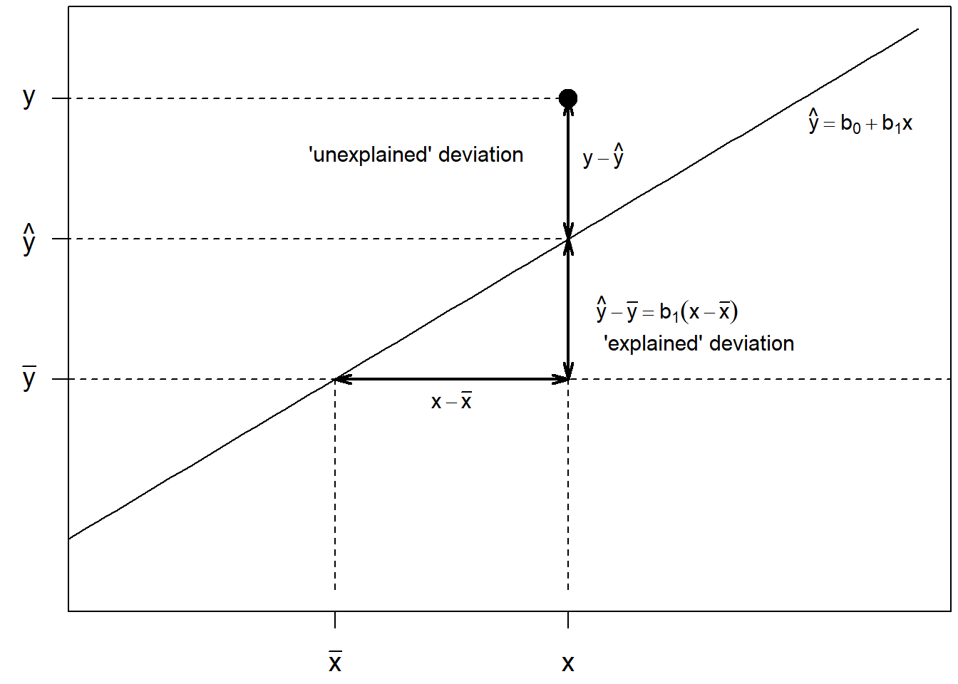

C, D and E Details. ANOVA Table

model_blr <- lm(sales ~ pop, data = Lot)
anova(model_blr)
sqrt(anova(model_blr)$Mean[2])
summary(model_blr)$r.squared

Analysis of Variance Table

Response: sales
          Df     Sum Sq    Mean Sq F value    Pr(>F)    
pop        1 2527165015 2527165015  175.77 < 2.2e-16 ***
Residuals 48  690116755   14377432                      
---
Signif. codes:  0 '***' 0.001 '**' 0.01 '*' 0.05 '.' 0.1 ' ' 1
[1] 3791.758
[1] 0.7854969

2.3.2 Exercise. Summarizing measures of uncertainty

Assignment Text

In a previous exercise, you developed a regression line to fit the variable medhome, the median house price for each zip code, as a predictor of lottery sales. The regression of medhome on sales has been summarized in the R object model_blr.

How reliable is the regression line? In this excercise, you will compute some of the standard measures that are used to summarize the goodness of this fit.

Instructions

Summarize the fitted regression model in an ANOVA table.
Determine the size of the typical residual, $s$.
Determine the coefficient of determination, $R^2$.

2.3.3 Exercise. Effects of linear transforms on measures of uncertainty

Assignment Text

Let us see how rescaling, a linear transformation, affects our measures of uncertainty. As before, the Wisconsin lottery dataset Wisc_lottery has been read into a dataframe Lot that also contains sales_1000, sales in thousands of dollars, and pop_1000, zip code population in thousands. How do measures of uncertainty change when going from the original units to thousands of those units?

Instructions

Run a regression of pop on sales_1000 and summarize this in an ANOVA table.
For this regression, determine the $s$ and the coefficient of determination, $R^2$.
Run a regression of pop_1000 on sales_1000 and summarize this in an ANOVA table.
For this regression, determine the $s$ and the coefficient of determination, $R^2$.

Hint. The residual standard error is also available as summary(model_blr1)$sigma. The coefficient of determination is also available as summary(model_blr1)$r.squared.

eyJsYW5ndWFnZSI6InIiLCJwcmVfZXhlcmNpc2VfY29kZSI6IiNMb3QgPC0gcmVhZC5jc3YoXCJDU1ZEYXRhXFxcXFdpc2NfbG90dGVyeS5jc3ZcIiwgaGVhZGVyID0gVFJVRSlcbkxvdCA8LSByZWFkLmNzdihcImh0dHBzOi8vYXNzZXRzLmRhdGFjYW1wLmNvbS9wcm9kdWN0aW9uL3JlcG9zaXRvcmllcy8yNjEwL2RhdGFzZXRzL2E3OTJiMzBmYjMyYjA4OTZkZDY4OTQ1MDFjYmFiMzJiNWQ0OGRmNTEvV2lzY19sb3R0ZXJ5LmNzdlwiLCBoZWFkZXIgPSBUUlVFKVxuTG90JHBvcF8xMDAwIDwtIExvdCRwb3AvMTAwMFxuTG90JHNhbGVzXzEwMDAgPC0gTG90JHNhbGVzLzEwMDAiLCJzYW1wbGUiOiIjIFJ1biBhIHJlZ3Jlc3Npb24gb2YgYHBvcGAgb24gYHNhbGVzXzEwMDBgIGFuZCBzdW1tYXJpemUgdGhpcyBpbiBhbiBBTk9WQSB0YWJsZS5cbm1vZGVsX2JscjEgPC0gbG0oc2FsZXNfMTAwMCAgfiBwb3AsIGRhdGEgPSBMb3QpXG5hbm92YShfX18pXG5cbiMgRGV0ZXJtaW5lIHRoZSAkcyQgYW5kIHRoZSBjb2VmZmljaWVudCBvZiBkZXRlcm1pbmF0aW9uLCAkUl4yJC4gIFxuc3FydChhbm92YShfX18pJE1lYW5bMl0pXG5zdW1tYXJ5KF9fXykkci5zcXVhcmVkXG5cbiMgUnVuIGEgcmVncmVzc2lvbiBvZiBgcG9wXzEwMDBgIG9uIGBzYWxlc18xMDAwYCBhbmQgc3VtbWFyaXplIHRoaXMgaW4gYW4gQU5PVkEgdGFibGUuXG5tb2RlbF9ibHIyIDwtIGxtKF9fXyAgfiBfX18sIGRhdGEgPSBMb3QpXG5hbm92YShtb2RlbF9ibHIyKVxuXG4jIERldGVybWluZSB0aGUgJHMkIGFuZCB0aGUgY29lZmZpY2llbnQgb2YgZGV0ZXJtaW5hdGlvbiwgJFJeMiQuIFxuX19fXG5fX18iLCJzb2x1dGlvbiI6Im1vZGVsX2JscjEgPC0gbG0oc2FsZXNfMTAwMCAgfiBwb3AsIGRhdGEgPSBMb3QpXG5hbm92YShtb2RlbF9ibHIxKVxuc3FydChhbm92YShtb2RlbF9ibHIxKSRNZWFuWzJdKVxuc3VtbWFyeShtb2RlbF9ibHIxKSRyLnNxdWFyZWRcbm1vZGVsX2JscjIgPC0gbG0oc2FsZXNfMTAwMCAgfiBwb3BfMTAwMCAsIGRhdGEgPSBMb3QpXG5hbm92YShtb2RlbF9ibHIyKVxuc3FydChhbm92YShtb2RlbF9ibHIyKSRNZWFuWzJdKVxuc3VtbWFyeShtb2RlbF9ibHIyKSRyLnNxdWFyZWQiLCJzY3QiOiJleCgpICU+JSBjaGVja19vYmplY3QoXCJtb2RlbF9ibHIxXCIsIHVuZGVmaW5lZF9tc2c9XCJQbGVhc2UgbmFtZSB0aGUgZmlyc3QgcmVncmVzc2lvbiBtb2RlbCBgbW9kZWxfYmxyMWAuXCIpICU+JSBjaGVja19lcXVhbChpbmNvcnJlY3RfbXNnPVwiUGxlYXNlIGRvIG5vdCBjaGFuZ2UgdGhpcyBzdGVwLCBpdCBzaG91bGQgcmVhZCBgbW9kZWxfYmxyMSA8LSBsbShzYWxlc18xMDAwIH4gcG9wLCBkYXRhID0gTG90KWAuXCIpXG5leCgpICU+JSBjaGVja19mdW5jdGlvbihcImFub3ZhXCIsIGluZGV4PTEsIG5vdF9jYWxsZWRfbXNnPVwiVXNlIGBhbm92YWAgdG8gc3VtbWFyaXplIHRoZSBmaXQgb2YgYG1vZGVsX2JscjFgLlwiKSAlPiUgY2hlY2tfcmVzdWx0KCkgJT4lIGNoZWNrX2VxdWFsKGluY29ycmVjdF9tc2c9XCJNYWtlIHN1cmUgdG8gc3BlY2lmeSB0aGF0IHdlIHdhbnQgdG8gcnVuIGBhbm92YWAgb24gYG1vZGVsX2JscjFgLlwiKVxuZXgoKSAlPiUgY2hlY2tfZnVuY3Rpb24oXCJzcXJ0XCIsIGluZGV4PTEsIG5vdF9jYWxsZWRfbXNnPVwiTWFrZSBzdXJlIHRvIHRha2UgdGhlIHNxdWFyZSByb290IGluIG9yZGVyIHRvIGZpbmQgYHNgLlwiKSAlPiUgY2hlY2tfcmVzdWx0KCkgJT4lIGNoZWNrX2VxdWFsKGluY29ycmVjdF9tc2c9XCJNYWtlIHN1cmUgeW91IGFyZSB0YWtpbmcgdGhlIHNxdWFyZSByb290IG9mIHRoZSBzZWNvbmQgYXJndW1lbnQgb2YgdGhlIG1lYW4gZm91bmQgdXNpbmcgYGFub3ZhYC5cIilcbmV4KCkgJT4lIGNoZWNrX2Z1bmN0aW9uKFwic3VtbWFyeVwiLCBpbmRleD0xLCBub3RfY2FsbGVkX21zZz1cIlVzZSBgc3VtbWFyeWAgdG8gZmluZCB0aGUgc3VtbWFyeSBzdGF0aXN0aWNzIG9mIGBtb2RlbF9ibHIxYC5cIikgJT4lIGNoZWNrX3Jlc3VsdCgpICU+JSBjaGVja19lcXVhbChpbmNvcnJlY3RfbXNnPVwiTWFrZSBzdXJlIHRvIHNwZWNpZnkgdGhhdCB3ZSB3YW50IHRoZSByLXNxdWFyZWQgdmFsdWUgZnJvbSBvdXIgbW9kZWwuXCIpXG5leCgpICU+JSBjaGVja19vYmplY3QoXCJtb2RlbF9ibHIyXCIsIHVuZGVmaW5lZF9tc2c9XCJQbGVhc2UgbmFtZSB0aGUgZmlyc3QgcmVncmVzc2lvbiBtb2RlbCBgbW9kZWxfYmxyMmAuXCIpICU+JSBjaGVja19lcXVhbChpbmNvcnJlY3RfbXNnPVwiTWFrZSBzdXJlIHRvIGNyZWF0ZSBgbW9kZWxfYmxyMmAgc3VjaCB0aGF0IGBzYWxlc18xMDAwYCBpcyBiYXNlZCBvbiBgcG9wXzEwMDBgLlwiKVxuZXgoKSAlPiUgY2hlY2tfZnVuY3Rpb24oXCJsbVwiLCBpbmRleD0yLCBub3RfY2FsbGVkX21zZz1cIm1ha2Ugc3VyZSB0byB1c2UgYGxtYCB0byBjcmVhdGUgYSByZWdyZXNzaW9uIG1vZGVsLlwiKSAlPiUge1xuICBjaGVja19hcmcoLiwgXCJmb3JtdWxhXCIpICU+JSBjaGVja19lcXVhbChpbmNvcnJlY3RfbXNnPVwibWFrZSBzdXJlIHRvIHNwZWNpZnkgd2Ugd291bGQgbGlrZSBgc2FsZXNfMTAwMGAgdG8gYmUgYmFzZWQgb24gYHBvcF8xMDAwYC5cIilcbiAgY2hlY2tfYXJnKC4sIFwiZGF0YVwiKSAlPiUgY2hlY2tfZXF1YWwoaW5jb3JyZWN0X21zZz1cIm1ha2Ugc3VyZSB0byBzcGVjaWZ5IHRoYXQgb3VyIGRhdGEgaXMgZnJvbSB0aGUgZGF0YWZyYW1lIGBMb3RgLlwiKVxufVxuZXgoKSAlPiUgY2hlY2tfZnVuY3Rpb24oXCJhbm92YVwiLGluZGV4PTMsbm90X2NhbGxlZF9tc2c9XCJVc2UgYGFub3ZhYCB0byBzdW1tYXJpemUgdGhlIGZpdCBvZiBgbW9kZWxfYmxyMmAuXCIpICU+JSBjaGVja19yZXN1bHQoKSAlPiUgY2hlY2tfZXF1YWwoaW5jb3JyZWN0X21zZz1cIk1ha2Ugc3VyZSB0byBzcGVjaWZ5IHRoYXQgd2Ugd2FudCB0byBydW4gYGFub3ZhYCBvbiBgbW9kZWxfYmxyMmAuXCIpXG5leCgpICU+JSBjaGVja19mdW5jdGlvbihcInNxcnRcIixpbmRleD0yLG5vdF9jYWxsZWRfbXNnPVwiTWFrZSBzdXJlIHRvIHRha2UgdGhlIHNxdWFyZSByb290IGluIG9yZGVyIHRvIGZpbmQgYHNgLlwiKSAlPiUgY2hlY2tfcmVzdWx0KCkgJT4lIGNoZWNrX2VxdWFsKGluY29ycmVjdF9tc2c9XCJNYWtlIHN1cmUgdGhhdCB5b3UgYXJlIHRha2luZyB0aGUgc3F1YXJlIHJvb3Qgb2YgdGhlIHNlY29uZCBhcmd1bWVudCBvZiB0aGUgbWVhbiBmb3VuZCB1c2luZyBgYW5vdmFgLlwiKVxuZXgoKSAlPiUgY2hlY2tfZnVuY3Rpb24oXCJhbm92YVwiLGluZGV4PTQsIG5vdF9jYWxsZWRfbXNnPVwibWFrZSBzdXJlIHRvIHJ1biBgYW5vdmFgIG9uIGBtb2RlbF9ibHIyYC5cIikgJT4lIGNoZWNrX3Jlc3VsdCgpICU+JSBjaGVja19lcXVhbChpbmNvcnJlY3RfbXNnPVwiTWFrZSBzdXJlIHRvIHNwZWNpZnkgdGhhdCB3ZSB3b3VsZCBsaWtlIHRvIHJ1biBgYW5vdmFgIG9uIGBtb2RlbF9ibHIyYC5cIilcbmV4KCkgJT4lIGNoZWNrX2Z1bmN0aW9uKFwic3VtbWFyeVwiLCBpbmRleD0yLCBub3RfY2FsbGVkX21zZz1cIlVzZSBgc3VtbWFyeWAgdG8gZmluZCB0aGUgc3VtbWFyeSBzdGF0cyBvbiBgbW9kZWxfYmxyMmAuXCIpICU+JSBjaGVja19yZXN1bHQoKSAlPiUgY2hlY2tfZXF1YWwoaW5jb3JyZWN0X21zZz1cIk1ha2Ugc3VyZSB0byBzcGVjaWZ5IHdlIHdhbnQgdGhlIHItc3F1YXJlZCB2YWx1ZSBmcm9tIG91ciBtb2RlbC5cIilcbnN1Y2Nlc3NfbXNnKFwiQ29uZ3JhdHVsYXRpb25zISBJbiB0aGlzIGV4ZXJjaXNlLCB5b3UgaGF2ZSBzZWVuIHRoYXQgcmVzY2FsaW5nIGRvZXMgbm90IGFmZmVjdCBvdXIgbWVhc3VyZXMgb2YgZ29vZG5lc3Mgb2YgZml0IGluIGFueSBtZWFuaW5nZnVsIHdheS4gRm9yIGV4YW1wbGUsIGNvZWZmY2llbnQgb2YgZGV0ZXJtaW5hdGlvbnMgYXJlIGNvbXBsZXRlbHkgdW5hZmZlY3RlZC4gVGhpcyBpcyBoZWxwZnVsIGJlY2F1c2Ugd2Ugd2lsbCByZXNjYWxlIHZhcmlhYmxlcyBleHRlbnNpdmVseSBpbiBvdXIgc2VhcmNoIGZvciBwYXR0ZXJucyBpbiB0aGUgZGF0YS5cIikiLCJoaW50IjoiVGhlIHJlc2lkdWFsIHN0YW5kYXJkIGVycm9yIGlzIGFsc28gYXZhaWxhYmxlIGFzIDxjb2RlPnN1bW1hcnkobW9kZWxfYmxyMSkkc2lnbWE8L2NvZGU+LiBUaGUgY29lZmZpY2llbnQgb2YgZGV0ZXJtaW5hdGlvbiBpcyBhbHNvIGF2YWlsYWJsZSBhcyA8Y29kZT5zdW1tYXJ5KG1vZGVsX2JscjEpJHIuc3F1YXJlZDwvY29kZT4uIn0=

2.4 Statistical inference

In this section, you learn how to:

Conduct a hypothesis test for a regression coefficient using either a rejection/acceptance procedure or a p-value
Calculate and interpret a confidence interval for a regression coefficient
Calculate and interpret a prediction interval at a specific value of a predictor variable

2.4.1 Video

Video Overhead Details

A Details. Summary of basic linear regression model

Introduce the output in the summary of the basic linear regression model.

Lot <- read.csv("CSVData\\Wisc_lottery.csv", header = TRUE)
#Lot <- read.csv("https://assets.datacamp.com/production/repositories/2610/datasets/a792b30fb32b0896dd6894501cbab32b5d48df51/Wisc_lottery.csv", header = TRUE)
#options(scipen = 8, digits = 4)
model_blr <- lm(sales ~ pop, data = Lot)
summary(model_blr)


Call:
lm(formula = sales ~ pop, data = Lot)

Residuals:
    Min      1Q  Median      3Q     Max 
-6046.7 -1460.9  -670.5   485.6 18229.5 

Coefficients:
             Estimate Std. Error t value Pr(>|t|)    
(Intercept) 469.70360  702.90619   0.668    0.507    
pop           0.64709    0.04881  13.258   <2e-16 ***
---
Signif. codes:  0 '***' 0.001 '**' 0.01 '*' 0.05 '.' 0.1 ' ' 1

Residual standard error: 3792 on 48 degrees of freedom
Multiple R-squared:  0.7855,    Adjusted R-squared:  0.781 
F-statistic: 175.8 on 1 and 48 DF,  p-value: < 2.2e-16

B Details. Hypothesis testing

> summary(model_blr)$coefficients
            Estimate Std. Error t value  Pr(>|t|)
(Intercept) 469.7036  702.90619  0.6682 5.072e-01
pop           0.6471    0.04881 13.2579 1.158e-17

C Details. Confidence intervals

confint(model_blr, level = .90)
confint(model_blr, level = .95)

                     5 %         95 %
(Intercept) -709.2276710 1648.6348666
pop            0.5652327    0.7289569
                   2.5 %     97.5 %
(Intercept) -943.5840183 1882.99121
pop            0.5489596    0.74523

D Details. Confidence intervals check

# Just for checking
summary(model_blr)$coefficients[2,1]
summary(model_blr)$coefficients[2,2]
qt(.975, 48)

summary(model_blr)$coefficients[2,1] - 
  summary(model_blr)$coefficients[2,2]*qt(.975, 48)

confint(model_blr, level = .95)
confint(model_blr, level = .95)

[1] 0.6470948
[1] 0.04880808
[1] 2.010635
[1] 0.5489596
                   2.5 %     97.5 %
(Intercept) -943.5840183 1882.99121
pop            0.5489596    0.74523
                   2.5 %     97.5 %
(Intercept) -943.5840183 1882.99121
pop            0.5489596    0.74523

E Details. Prediction intervals

NewData <- data.frame(pop = 10000)
predict(model_blr, NewData, interval = "prediction", level = .90)
predict(model_blr, NewData, interval = "prediction", level = .99)

       fit      lwr      upr
1 6940.651 517.4933 13363.81
       fit       lwr      upr
1 6940.651 -3331.214 17212.52

2.4.2 Exercise. Statistical inference and Wisconsin lottery

Assignment Text

In a previous exercise, you developed a regression line with the variable medhome, the median house price for each zip code, as a predictor of lottery sales. The regression of medhome on sales has been summarized in the R object model_blr.

This exercise allows you to practice the standard inferential tasks: hypothesis testing, confidence intervals, and prediction.

Instructions

Summarize the regression model and identify the t-statistic for testing the importance of the regression coefficient associated with medhome.
Use the function confint() to provide a 95% confidence interval for the regression coefficient associated with medhome.
Consider a zip code with a median housing price equal to 50 (in thousands of dollars). Use the function predict() to provide a point prediction and a 95% prediction interval for sales.

eyJsYW5ndWFnZSI6InIiLCJwcmVfZXhlcmNpc2VfY29kZSI6IiNMb3QgPC0gcmVhZC5jc3YoXCJDU1ZEYXRhXFxcXFdpc2NfbG90dGVyeS5jc3ZcIiwgaGVhZGVyID0gVFJVRSlcbkxvdCA8LSByZWFkLmNzdihcImh0dHBzOi8vYXNzZXRzLmRhdGFjYW1wLmNvbS9wcm9kdWN0aW9uL3JlcG9zaXRvcmllcy8yNjEwL2RhdGFzZXRzL2E3OTJiMzBmYjMyYjA4OTZkZDY4OTQ1MDFjYmFiMzJiNWQ0OGRmNTEvV2lzY19sb3R0ZXJ5LmNzdlwiLCBoZWFkZXIgPSBUUlVFKSIsInNhbXBsZSI6Im1vZGVsX2JscjEgPC0gbG0oc2FsZXMgfiBtZWRob21lLCBkYXRhID0gTG90KVxuIyBTdW1tYXJpemUgdGhlIHJlZ3Jlc3Npb24gbW9kZWwgYW5kIGlkZW50aWZ5IHRoZSAkdCQtc3RhdGlzdGljIGZvciB0ZXN0aW5nIHRoZSBpbXBvcnRhbmNlIG9mIHRoZSByZWdyZXNzaW9uIGNvZWZmaWNpZW50IGFzc29jaWF0ZWQgd2l0aCBgbWVkaG9tZWAuXG5zdW1tYXJ5KF9fXylcbnN1bW1hcnkoX19fKSRjb2VmZmljaWVudHNcbnN1bW1hcnkoX19fKSRjb2VmZmljaWVudHNbLDNdXG5cbiMgUHJvdmlkZSBhIDk1XFwlIGNvbmZpZGVuY2UgaW50ZXJ2YWwgZm9yIHRoZSByZWdyZXNzaW9uIGNvZWZmaWNpZW50IGFzc29jaWF0ZWQgd2l0aCBgbWVkaG9tZWAuXG5jb25maW50KF9fXywgbGV2ZWwgPSBfX18pXG5cbiMgUHJvdmlkZSBhIHBvaW50IHByZWRpY3Rpb24gYW5kIGEgOTVcXCUgcHJlZGljdGlvbiBpbnRlcnZhbCBmb3Igc2FsZXMuXG5OZXdEYXRhMSA8LSBkYXRhLmZyYW1lKG1lZGhvbWUgPSA1MClcbnByZWRpY3QoX19fLCBOZXdEYXRhMSwgaW50ZXJ2YWwgPSBcInByZWRpY3Rpb25cIiwgbGV2ZWwgPSBfX18pIiwic29sdXRpb24iOiJtb2RlbF9ibHIxIDwtIGxtKHNhbGVzIH4gbWVkaG9tZSwgZGF0YSA9IExvdClcbnN1bW1hcnkobW9kZWxfYmxyMSlcbnN1bW1hcnkobW9kZWxfYmxyMSkkY29lZmZpY2llbnRzXG5zdW1tYXJ5KG1vZGVsX2JscjEpJGNvZWZmaWNpZW50c1ssM11cblxuY29uZmludChtb2RlbF9ibHIxLCBsZXZlbCA9IC45NSlcblxuTmV3RGF0YTEgPC0gZGF0YS5mcmFtZShtZWRob21lID0gNTApXG5wcmVkaWN0KG1vZGVsX2JscjEsIE5ld0RhdGExLCBpbnRlcnZhbCA9IFwicHJlZGljdGlvblwiLCBsZXZlbCA9IC45NSkiLCJzY3QiOiJleCgpICU+JSBjaGVja19vYmplY3QoXCJtb2RlbF9ibHIxXCIsdW5kZWZpbmVkX21zZz1cIk1ha2Ugc3VyZSB0aGUgZmlyc3QgcmVncmVzc2lvbiBtb2RlbCBpcyBuYW1lZCBgbW9kZWxfYmxyMWAuXCIpICU+JSBjaGVja19lcXVhbChpbmNvcnJlY3RfbXNnPVwiTWFrZSBzdXJlIHRoYXQgYG1vZGVsX2JscjFgIGlzIGNyZWF0ZWQgYnkgbW9kZWxpbmcgYHNhbGVzYCBiYXNlZCBvbiBgbWVkaG9tZWAuXCIpXG5leCgpICU+JSBjaGVja19mdW5jdGlvbihcImxtXCIsbm90X2NhbGxlZF9tc2c9XCJNYWtlIHN1cmUgdG8gdXNlIGBsbWAgdG8gY3JlYXRlIGEgbGluZWFyIG1vZGVsLiBcIikgJT4lIHtcbiAgY2hlY2tfYXJnKC4sIFwiZm9ybXVsYVwiKSAlPiUgY2hlY2tfZXF1YWwoaW5jb3JyZWN0X21zZz1cIk1ha2Ugc3VyZSB0byBjcmVhdGUgYSBtb2RlbCBzbyB0aGF0IGBzYWxlc2AgYXJlIGJhc2VkIG9uIGBtZWRob21lYC5cIilcbiAgY2hlY2tfYXJnKC4sIFwiZGF0YVwiKSAlPiUgY2hlY2tfZXF1YWwoaW5jb3JyZWN0X21zZz1cIk1ha2Ugc3VyZSB0byBzcGVjaWZ5IHRoYXQgb3VyIGRhdGEgY29tZXMgZnJvbSBgTG90YC5cIilcbn1cbmV4KCkgJT4lIGNoZWNrX2Z1bmN0aW9uKFwic3VtbWFyeVwiLGluZGV4PTEsbm90X2NhbGxlZF9tc2c9XCJQbGVhc2UgdXNlIGBzdW1tYXJ5YCB0byBmaW5kIHN1bW1hcnkgcmVzdWx0cy4gXCIpICU+JSBjaGVja19hcmcoXCJvYmplY3RcIikgJT4lIGNoZWNrX2VxdWFsKGluY29ycmVjdF9tc2c9XCJNYWtlIHN1cmUgdG8gc3BlY2lmeSB3ZSB3YW50IHRvIHRha2UgdGhlIHN1bW1hcnkgb2YgYG1vZGVsX2JscjFgLlwiKVxuZXgoKSAlPiUgY2hlY2tfZnVuY3Rpb24oXCJzdW1tYXJ5XCIsaW5kZXg9Mixub3RfY2FsbGVkX21zZz1cIlBsZWFzZSB1c2UgYHN1bW1hcnlgIHRvIGZpbmQgc3VtbWFyeSByZXN1bHRzLiBcIikgJT4lIGNoZWNrX3Jlc3VsdCgpICU+JSBjaGVja19lcXVhbChpbmNvcnJlY3RfbXNnPVwiTWFrZSBzdXJlIHRvIHNwZWNpZnkgd2Ugd2FudCB0byBmaW5kIHRoZSBjb2VmZmljaWVudHMgdXNpbmcgdGhlIHN1bW1hcnkgb2YgYG1vZGVsX2JscjFgLlwiKVxuZXgoKSAlPiUgY2hlY2tfZnVuY3Rpb24oXCJzdW1tYXJ5XCIsaW5kZXg9Myxub3RfY2FsbGVkX21zZz1cIlBsZWFzZSB1c2UgYHN1bW1hcnlgIHRvIGZpbmQgc3VtbWFyeSByZXN1bHRzLiBcIikgJT4lIGNoZWNrX3Jlc3VsdCgpICU+JSBjaGVja19lcXVhbChpbmNvcnJlY3RfbXNnPVwiTWFrZSBzdXJlIHRvIHNwZWNpZnkgd2Ugd2FudCB0byBmaW5kIHRoZSB0LXN0YXQgdXNpbmcgdGhlIHN1bW1hcnkgb2YgYG1vZGVsX2JscjFgLlwiIClcbmV4KCkgJT4lIGNoZWNrX2Z1bmN0aW9uKFwiY29uZmludFwiLG5vdF9jYWxsZWRfbXNnPVwiTWFrZSBzdXJlIHRvIHVzZSBgY29uZmludGAgdG8gY3JlYXRlIGEgY29uZmlkZW5jZSBpbnRlcnZhbC4gXCIpICU+JSB7XG4gIGNoZWNrX2FyZyguLCBcIm9iamVjdFwiKSAlPiUgY2hlY2tfZXF1YWwoaW5jb3JyZWN0X21zZz1cIk1ha2Ugc3VyZSB0byBzcGVjaWZ5IHRoYXQgd2Ugd2FudCB0byB1c2UgYG1vZGVsX2JscjFgIHRvIGNyZWF0ZSBvdXIgaW50ZXJ2YWwuXCIpXG4gIGNoZWNrX2FyZyguLCBcImxldmVsXCIpICU+JSBjaGVja19lcXVhbChpbmNvcnJlY3RfbXNnPVwiTWFrZSBzdXJlIHRvIHNwZWNpZnkgd2Ugd2FudCBhIDk1JSBjb25maWRlbmNlIGludGVydmFsLiBcIilcbn1cbmV4KCkgJT4lIGNoZWNrX2Z1bmN0aW9uKFwiY29uZmludFwiKSAlPiUgY2hlY2tfcmVzdWx0KCkgJT4lIGNoZWNrX2VxdWFsKClcbmV4KCkgJT4lIGNoZWNrX29iamVjdChcIk5ld0RhdGExXCIsdW5kZWZpbmVkX21zZz1cIk1ha2UgbmV3IGRhdGEgdXNpbmcgYE5ld0RhdGExYCBhcyB0aGUgbmFtZSBvZiB0aGUgZGF0YWZyYW1lLiBcIikgJT4lIGNoZWNrX2VxdWFsKGluY29ycmVjdF9tc2c9XCJNYWtlIHN1cmUgdG8gc3BlY2lmeSBgbWVkaG9tZT01MGAuXCIpXG5leCgpICU+JSBjaGVja19mdW5jdGlvbihcInByZWRpY3RcIiwgbm90X2NhbGxlZF9tc2c9XCJVc2UgYHByZWRpY3RgIHRvIGNyZWF0ZSBwcmVkaWN0aW9uIGludGVydmFscyB1c2luZyBvdXIgbW9kZWwgYW5kIG91ciBuZXcgZGF0YS4gXCIpICU+JSB7XG4gIGNoZWNrX2FyZyguLCBcIm9iamVjdFwiKSAlPiUgY2hlY2tfZXF1YWwoaW5jb3JyZWN0X21zZz1cIk1ha2Ugc3VyZSB0byBzcGVjaWZ5IHdlIHdhbnQgdG8gdXNlIGBtb2RlbF9ibHIxYC5cIilcbiAgY2hlY2tfYXJnKC4sIFwibmV3ZGF0YVwiKSAlPiUgY2hlY2tfZXF1YWwoaW5jb3JyZWN0X21zZz1cIk1ha2Ugc3VyZSB0byBzcGVjaWZ5IHdlIHdhbnQgdG8gdXNlIGBOZXdEYXRhMWAgYXMgb3VyIG5ld2RhdGEuIFwiKVxuICBjaGVja19hcmcoLiwgXCJpbnRlcnZhbFwiKSAlPiUgY2hlY2tfZXF1YWwoaW5jb3JyZWN0X21zZz1cIk1ha2Ugc3VyZSB0byBzcGVjaWZ5IHRoYXQgYGludGVydmFsYCBzaG91bGQgZXF1YWwgYHByZWRpY3Rpb25gLlwiKVxuICBjaGVja19hcmcoLiwgXCJsZXZlbFwiKSAlPiUgY2hlY2tfZXF1YWwoaW5jb3JyZWN0X21zZz1cIk1ha2Ugc3VyZSB0byBzcGVjaWZ5IHRoYXQgd2Ugd291bGQgbGlrZSBhIDk1JSBwcmVkaWN0aW9uIGludGVydmFsLiBcIilcbn1cbmV4KCkgJT4lIGNoZWNrX2Z1bmN0aW9uKFwicHJlZGljdFwiKSAlPiUgY2hlY2tfcmVzdWx0KCkgJT4lIGNoZWNrX2VxdWFsKClcbnN1Y2Nlc3NfbXNnKFwiQ29uZ3JhdHVsYXRpb25zISBNdWNoIG9mIHdoYXQgd2UgbGVhcm4gZnJvbSBhIGRhdGEgbW9kZWxpbmcgZXhlcmNpc2UgY2FuIGJlIHN1bW1hcml6ZWQgdXNpbmcgc3RhbmRhcmQgaW5mZXJlbnRpYWwgdG9vbHM6IGh5cG90aGVzaXMgdGVzdGluZywgY29uZmlkZW5jZSBpbnRlcnZhbHMsIGFuZCBwcmVkaWN0aW9uLlwiKSIsImhpbnQiOiJUYWtpbmcgYSBbc3VtbWFyeSgpXSBvZiBhIHJlZ3Jlc3Npb24gb2JqZWN0IHByb2R1Y2VzIGEgbmV3IG9iamVlY3QuIFlvdSBjYW4gdXNlIHRoZSBbc3RyKCldIHN0cnVjdHVyZSBjb21tYW5kIHRvIGxlYXJuIG1vcmUgYWJvdXQgdGhlIG5ldyBvYmplY3QuIFRyeSBvdXQgYSBjb21tYW5kIHN1Y2ggYXMgPGNvZGU+c3RyKHN1bW1hcnkobW9kZWxfYmxyKSk8L2NvZGU+In0=

2.5 Diagnostics

In this section, you learn how to:

Describe how diagnostic checking and residual analysis are used in a statistical analysis
Describe several model misspecifications commonly encountered in a regression analysis

2.5.1 Video

Video Overhead Details

A Details. Unusual observations in regression

We have defined regression estimates as minimizers of a least squares objective function.
An appealing intuitive feature of linear regressions is that regression estimates can be expressed as weighted averages of outcomes.
The weights vary by observation, some observations are more important than others.
“Unusual” observations are far from the majority of the data set:
- Unusual in the vertical direction is called an outlier.
- Unusual in the horizontal directional is called a high leverage point.

B Details. Example. Outliers and High Leverage Points

outlr <- read.csv("CSVData\\Outlier.csv", header = TRUE)

#  FIGURE 2.7
plot(outlr$x, outlr$y, xlim = c(0, 10), ylim = c(2, 9), xlab = "x", ylab = "y")
text(4.5, 8.0, "A")
text(9.8, 8.0, "B")
text(9.8, 2.5, "C")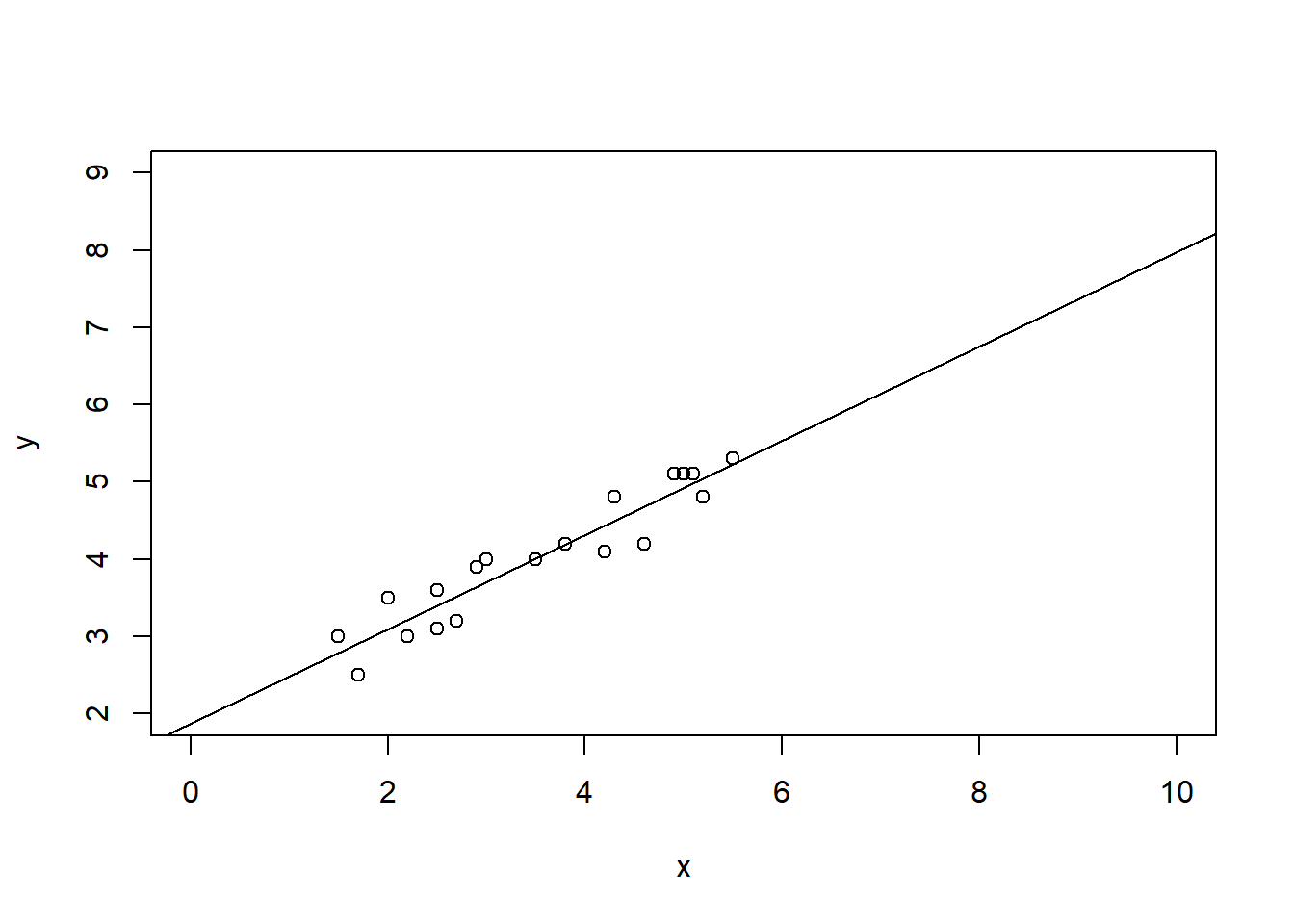

C Details. Regression fit with 19 base observations

model_outlr0 <- lm(y ~ x, data = outlr, subset = -c(20,21,22))
summary(model_outlr0)
plot(outlr$x[1:19], outlr$y[1:19], xlab = "x", ylab = "y", xlim = c(0, 10), ylim = c(2, 9))
abline(model_outlr0)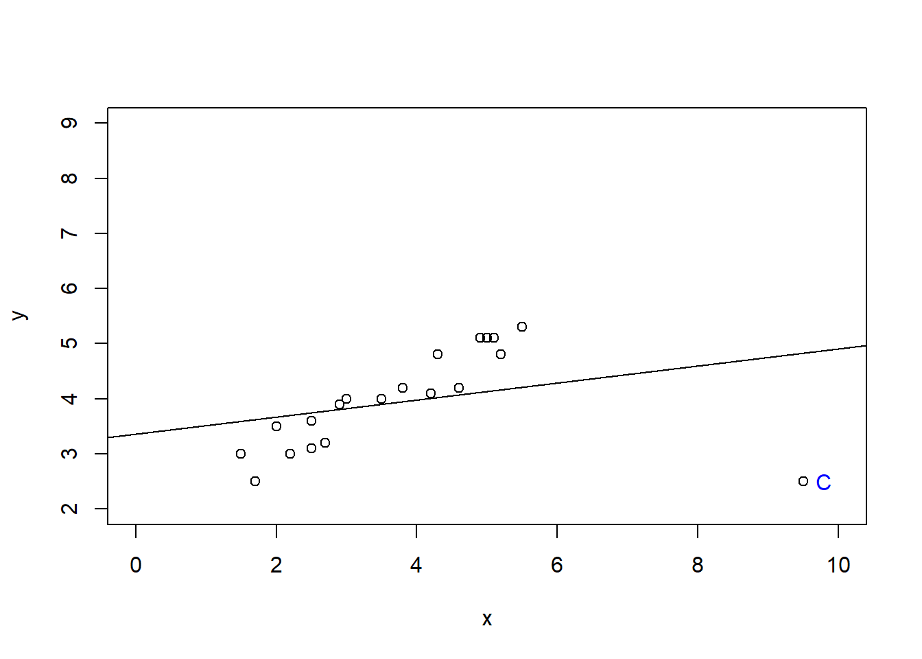


Call:
lm(formula = y ~ x, data = outlr, subset = -c(20, 21, 22))

Residuals:
    Min      1Q  Median      3Q     Max 
-0.4790 -0.2708  0.0711  0.2263  0.4094 

Coefficients:
            Estimate Std. Error t value Pr(>|t|)    
(Intercept)  1.86874    0.19583   9.543 3.06e-08 ***
x            0.61094    0.05219  11.705 1.47e-09 ***
---
Signif. codes:  0 '***' 0.001 '**' 0.01 '*' 0.05 '.' 0.1 ' ' 1

Residual standard error: 0.2883 on 17 degrees of freedom
Multiple R-squared:  0.8896,    Adjusted R-squared:  0.8831 
F-statistic:   137 on 1 and 17 DF,  p-value: 1.471e-09

D Details. Regression fit with 19 base observations plus C

model_outlrC <- lm(y ~ x, data = outlr, subset = -c(20,21))
summary(model_outlrC)
plot(outlr$x[c(1:19,22)], outlr$y[c(1:19,22)], xlab = "x", ylab = "y", xlim = c(0, 10), ylim = c(2, 9))
text(9.8, 2.5, "C", col = "blue")
abline(model_outlrC)


Call:
lm(formula = y ~ x, data = outlr, subset = -c(20, 21))

Residuals:
     Min       1Q   Median       3Q      Max 
-2.32947 -0.57819  0.09772  0.67240  1.09097 

Coefficients:
            Estimate Std. Error t value Pr(>|t|)    
(Intercept)   3.3559     0.4560   7.360 7.87e-07 ***
x             0.1551     0.1078   1.439    0.167    
---
Signif. codes:  0 '***' 0.001 '**' 0.01 '*' 0.05 '.' 0.1 ' ' 1

Residual standard error: 0.8648 on 18 degrees of freedom
Multiple R-squared:  0.1031,    Adjusted R-squared:  0.0533 
F-statistic:  2.07 on 1 and 18 DF,  p-value: 0.1674

E Details. R code

model_outlr0 <- lm(y ~ x, data = outlr, subset = -c(20,21,22))
summary(model_outlr0)
model_outlrA <- lm(y ~ x, data = outlr, subset = -c(21,22))
summary(model_outlrA)
model_outlrB <- lm(y ~ x, data = outlr, subset = -c(20,22))
summary(model_outlrB)
model_outlrC <- lm(y ~ x, data = outlr, subset = -c(20,21))
summary(model_outlrC)


Call:
lm(formula = y ~ x, data = outlr, subset = -c(20, 21, 22))

Residuals:
    Min      1Q  Median      3Q     Max 
-0.4790 -0.2708  0.0711  0.2263  0.4094 

Coefficients:
            Estimate Std. Error t value Pr(>|t|)    
(Intercept)  1.86874    0.19583   9.543 3.06e-08 ***
x            0.61094    0.05219  11.705 1.47e-09 ***
---
Signif. codes:  0 '***' 0.001 '**' 0.01 '*' 0.05 '.' 0.1 ' ' 1

Residual standard error: 0.2883 on 17 degrees of freedom
Multiple R-squared:  0.8896,    Adjusted R-squared:  0.8831 
F-statistic:   137 on 1 and 17 DF,  p-value: 1.471e-09


Call:
lm(formula = y ~ x, data = outlr, subset = -c(21, 22))

Residuals:
    Min      1Q  Median      3Q     Max 
-0.7391 -0.3928 -0.1805  0.1225  3.2689 

Coefficients:
            Estimate Std. Error t value Pr(>|t|)    
(Intercept)   1.7500     0.5736   3.051 0.006883 ** 
x             0.6933     0.1517   4.570 0.000237 ***
---
Signif. codes:  0 '***' 0.001 '**' 0.01 '*' 0.05 '.' 0.1 ' ' 1

Residual standard error: 0.8455 on 18 degrees of freedom
Multiple R-squared:  0.5371,    Adjusted R-squared:  0.5114 
F-statistic: 20.89 on 1 and 18 DF,  p-value: 0.0002374


Call:
lm(formula = y ~ x, data = outlr, subset = -c(20, 22))

Residuals:
     Min       1Q   Median       3Q      Max 
-0.51763 -0.28094  0.03452  0.23586  0.44581 

Coefficients:
            Estimate Std. Error t value Pr(>|t|)    
(Intercept)  1.77463    0.15020   11.81 6.48e-10 ***
x            0.63978    0.03551   18.02 5.81e-13 ***
---
Signif. codes:  0 '***' 0.001 '**' 0.01 '*' 0.05 '.' 0.1 ' ' 1

Residual standard error: 0.2849 on 18 degrees of freedom
Multiple R-squared:  0.9474,    Adjusted R-squared:  0.9445 
F-statistic: 324.5 on 1 and 18 DF,  p-value: 5.808e-13


Call:
lm(formula = y ~ x, data = outlr, subset = -c(20, 21))

Residuals:
     Min       1Q   Median       3Q      Max 
-2.32947 -0.57819  0.09772  0.67240  1.09097 

Coefficients:
            Estimate Std. Error t value Pr(>|t|)    
(Intercept)   3.3559     0.4560   7.360 7.87e-07 ***
x             0.1551     0.1078   1.439    0.167    
---
Signif. codes:  0 '***' 0.001 '**' 0.01 '*' 0.05 '.' 0.1 ' ' 1

Residual standard error: 0.8648 on 18 degrees of freedom
Multiple R-squared:  0.1031,    Adjusted R-squared:  0.0533 
F-statistic:  2.07 on 1 and 18 DF,  p-value: 0.1674

F Details. Visualizing four regression fits

plot(outlr$x, outlr$y, xlim = c(0, 10), ylim = c(2, 9), xlab = "x", ylab = "y")
text(4.5, 8.0, "A", col = "red")
text(9.8, 8.0, "B", col = "green")
text(9.8, 2.5, "C", col = "blue")
abline(model_outlr0)
abline(model_outlrA, col = "red")
abline(model_outlrB, col = "green")
abline(model_outlrC, col = "blue")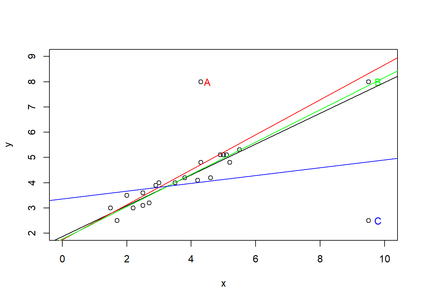

G Details. Results from four regression models

\[\begin{matrix} \begin{array}{c} \text{Results from Four Regressions} \end{array}\\\scriptsize \begin{array}{l|rrrrr} \hline \text{Data} & b_0 & b_1 & s & R^2(\%) & t(b_1) \\ \hline \text{19 Base Points} & 1.869 & 0.611 & 0.288 & 89.0 & 11.71 \\ \text{19 Base Points} ~+~ A & 1.750 & 0.693 & 0.846 & 53.7 & 4.57 \\ \text{19 Base Points} ~+~ B & 1.775 & 0.640 & 0.285 & 94.7 & 18.01 \\ \text{19 Base Points} ~+~ C & 3.356 & 0.155 & 0.865 & 10.3 & 1.44 \\ \hline \end{array} \end{matrix}\]

2.5.2 Exercise. Assessing outliers in lottery sales

Assignment Text

In an earlier video, we made a scatter plot of population versus sales. This plot exhibits an outlier; the point in the upper left-hand side of the plot represents a zip code that includes Kenosha, Wisconsin. Sales for this zip code are unusually high given its population.

This exercise summarizes the regression fit both with and without this zip code in order to see how robust our results are to the inclusion of this unusual observation.

Instructions

A basic linear regression fit of population on sales has already been fit in the object model_blr. Re-fit this same model to the data, this time omitting Kenosha (observation number 9).
Plot these two least squares fitted lines superimposed on the full data set.
What is the effect on the distribution of residuals by removing this point? Calculate a normal qq plot with and without Kenosha.

eyJsYW5ndWFnZSI6InIiLCJwcmVfZXhlcmNpc2VfY29kZSI6IiNMb3QgPC0gcmVhZC5jc3YoXCJDU1ZEYXRhXFxcXFdpc2NfbG90dGVyeS5jc3ZcIiwgaGVhZGVyID0gVFJVRSlcbkxvdCA8LSByZWFkLmNzdihcImh0dHBzOi8vYXNzZXRzLmRhdGFjYW1wLmNvbS9wcm9kdWN0aW9uL3JlcG9zaXRvcmllcy8yNjEwL2RhdGFzZXRzL2E3OTJiMzBmYjMyYjA4OTZkZDY4OTQ1MDFjYmFiMzJiNWQ0OGRmNTEvV2lzY19sb3R0ZXJ5LmNzdlwiLCBoZWFkZXIgPSBUUlVFKSIsInNhbXBsZSI6Im1vZGVsX2JsciA8LWxtKHNhbGVzIH4gcG9wLCBkYXRhID0gTG90KVxuc3VtbWFyeShtb2RlbF9ibHIpXG4jIFJlLWZpdCB0aGlzIG1vZGVsIHRvIHRoZSBkYXRhLCB0aGlzIHRpbWUgb21pdHRpbmcgS2Vub3NoYSAob2JzZXJ2YXRpb24gbnVtYmVyIDkpLlxubW9kZWxfS2Vub3NoYSA8LSBsbShfX18gfiBfX18sIGRhdGEgPSBMb3QsIHN1YnNldCA9IC1jKDkpKVxuc3VtbWFyeShfX18pXG5cbiMgUGxvdCB0aGVzZSB0d28gbGVhc3Qgc3F1YXJlcyBmaXR0ZWQgbGluZXMgc3VwZXJpbXBvc2VkIG9uIHRoZSBmdWxsIGRhdGEgc2V0LlxucGxvdChfX18sIF9fXywgeGxhYiA9IFwicG9wdWxhdGlvblwiLCB5bGFiID0gXCJzYWxlc1wiKVxudGV4dCg1MDAwLCAyNDAwMCwgXCJLZW5vc2hhXCIpXG5hYmxpbmUobW9kZWxfYmxyLCBjb2w9XCJibHVlXCIpXG5hYmxpbmUoX19fLCBjb2w9XCJyZWRcIilcblxuIyBDYWxjdWxhdGUgYSBub3JtYWwgcXEgcGxvdCB3aXRoIGFuZCB3aXRob3V0IEtlbm9zaGEuXG5wYXIobWZyb3cgPSBjKDEsIDIpKVxucXFub3JtKHJlc2lkdWFscyhfX18pLCBtYWluID0gXCJcIilcbnFxbGluZShyZXNpZHVhbHMoX19fKSkpXG5xcW5vcm0ocmVzaWR1YWxzKF9fXykpLCBtYWluID0gXCJcIilcbnFxbGluZShyZXNpZHVhbHMoX19fKSkpIiwic29sdXRpb24iOiJtb2RlbF9ibHIgPC1sbShzYWxlcyB+IHBvcCwgZGF0YSA9IExvdClcbnN1bW1hcnkobW9kZWxfYmxyKVxubW9kZWxfS2Vub3NoYSA8LSBsbShzYWxlcyB+IHBvcCwgZGF0YSA9IExvdCwgc3Vic2V0ID0gLWMoOSkpXG5zdW1tYXJ5KG1vZGVsX0tlbm9zaGEpXG5cbnBsb3QoTG90JHBvcCwgTG90JHNhbGVzLCB4bGFiID0gXCJwb3B1bGF0aW9uXCIsIHlsYWIgPSBcInNhbGVzXCIpXG50ZXh0KDUwMDAsIDI0MDAwLCBcIktlbm9zaGFcIilcbmFibGluZShtb2RlbF9ibHIsIGNvbD1cImJsdWVcIilcbmFibGluZShtb2RlbF9LZW5vc2hhLCBjb2w9XCJyZWRcIilcblxucGFyKG1mcm93ID0gYygxLCAyKSlcbnFxbm9ybShyZXNpZHVhbHMobW9kZWxfYmxyKSwgbWFpbiA9IFwiXCIpXG5xcWxpbmUocmVzaWR1YWxzKG1vZGVsX2JscikpXG5xcW5vcm0ocmVzaWR1YWxzKG1vZGVsX0tlbm9zaGEpLCBtYWluID0gXCJcIilcbnFxbGluZShyZXNpZHVhbHMobW9kZWxfS2Vub3NoYSkpIiwic2N0IjoiZXgoKSAlPiUgY2hlY2tfb2JqZWN0KFwibW9kZWxfYmxyXCIsIHVuZGVmaW5lZF9tc2c9XCJNYWtlIHN1cmUgdG8gbmFtZSB0aGUgZmlyc3QgcmVncmVzc2lvbiBtb2RlbCBgbW9kZWxfYmxyYC5cIikgJT4lIGNoZWNrX2VxdWFsKGluY29ycmVjdF9tc2c9XCJUaGlzIGhhcyBhbHJlYWR5IGJlZW4gYm9uZSBmb3IgeW91LCBwbGVhc2UgZG8gbm90IGNoYW5nZSBpdC5cIilcbmV4KCkgJT4lIGNoZWNrX2Z1bmN0aW9uKFwibG1cIiwgaW5kZXg9MSwgbm90X2NhbGxlZF9tc2c9XCJVc2UgYGxtYCB0byBjcmVhdGUgdGhlIGxpbmVhciBtb2RlbCBmb3IgYG1vZGVsX2JscmAuXCIpICU+JSB7XG4gIGNoZWNrX2FyZyguLCBcImZvcm11bGFcIikgJT4lIGNoZWNrX2VxdWFsKGluY29ycmVjdF9tc2c9XCJNYWtlIHN1cmUgdG8gbW9kZWwgYHNhbGVzYCBiYXNlZCBvbiBgcG9wYC5cIilcbiAgY2hlY2tfYXJnKC4sIFwiZGF0YVwiKSAlPiUgY2hlY2tfZXF1YWwoaW5jb3JyZWN0X21zZz1cIk1ha2Ugc3VyZSB0byBzcGVjaWZ5IHRoZSBkYXRhZnJhbWUgd2UgYXJlIHVzaW5nLCBgTG90YC5cIilcbn1cbmV4KCkgJT4lIGNoZWNrX2Z1bmN0aW9uKFwic3VtbWFyeVwiLCBpbmRleD0xLCBub3RfY2FsbGVkX21zZz1cInJ1biBgc3VtbWFyeWAgb24gYG1vZGVsX2JscmAuXCIpICU+JSBjaGVja19hcmcoLiwgXCJvYmplY3RcIikgJT4lIGNoZWNrX2VxdWFsKGluY29ycmVjdF9tc2c9XCJNYWtlIHN1cmUgdG8gc3BlY2lmeSB0aGF0IHdlIHdhbnQgdGhlIHN1bW1hcnkgb2YgYG1vZGVsX2JscmAuXCIpXG5leCgpICU+JSBjaGVja19vYmplY3QoXCJtb2RlbF9LZW5vc2hhXCIsIHVuZGVmaW5lZF9tc2c9XCJOYW1lIHRoZSByZXN1bHQgb2YgYSBgbG1gIGV4Y2x1ZGluZyBLZW5vc2hhIGBtb2RlbF9LZW5vc2hhYC5cIikgJT4lIGNoZWNrX2VxdWFsKGluY29ycmVjdF9tc2c9XCJNYWtlIHN1cmUgdG8gZXhjbHVkZSBvYnNlcnZhdGlvbiA5LlwiKVxuZXgoKSAlPiUgY2hlY2tfZnVuY3Rpb24oXCJsbVwiLCBpbmRleD0yLCBub3RfY2FsbGVkX21zZz1cIkNyZWF0ZSBhIGxpbmVhciBtb2RlbCBleGNsdWRpbmcgdGhlIEtlbm9zaGEgb2JzZXJ2YXRpb24uXCIpICU+JSB7XG4gIGNoZWNrX2FyZyguLCBcImZvcm11bGFcIikgJT4lIGNoZWNrX2VxdWFsKGluY29ycmVjdF9tc2c9XCJNYWtlIHN1cmUgdG8gc3BlY2lmeSB0aGF0IHdlIHdhbnQgdG8gYmFzZSBgc2FsZXNgIG9uIGBwb3BgLlwiKVxuICBjaGVja19hcmcoLiwgXCJkYXRhXCIpICU+JSBjaGVja19lcXVhbChpbmNvcnJlY3RfbXNnPVwiTWFrZSBzdXJlIHRvIHNwZWNpZnkgdGhhdCBvdXIgZGF0YSBpcyBmcm9tIHRoZSBkYXRhZnJhbWUgYExvdGAuXCIpXG4gIGNoZWNrX2FyZyguLCBcInN1YnNldFwiKSAlPiUgY2hlY2tfZXF1YWwoaW5jb3JyZWN0X21zZz1cIk1ha2Ugc3VyZSB0byByZW1vdmUgdGhlIEtlbm9zaGEgb2JzZXJ2YXRpb24gZnJvbSB0aGUgZGF0YS4gS2Vub3NoYSBpcyBvYnNlcnZhdGlvbiA5LlwiKVxufVxuZXgoKSAlPiUgY2hlY2tfZnVuY3Rpb24oXCJzdW1tYXJ5XCIsIGluZGV4PTIsIG5vdF9jYWxsZWRfbXNnPVwiTG9vayBhdCB0aGUgc3VtbWFyeSBzdGF0cyBvZiBgbW9kZWxfS2Vub3NoYWAgdXNpbmcgYHN1bW1hcnlgLlwiKSAlPiUgY2hlY2tfYXJnKC4sIFwib2JqZWN0XCIpICU+JSBjaGVja19lcXVhbChpbmNvcnJlY3RfbXNnPVwiTWFrZSBzdXJlIHRvIHNwZWNpZnkgd2Ugd2FudCBzdW1tYXJ5IHN0YXRzIG9mIGBtb2RlbF9LZW5vc2hhYC5cIiApXG5leCgpICU+JSBjaGVja19mdW5jdGlvbihcInBsb3RcIiwgbm90X2NhbGxlZF9tc2c9XCJDcmVhdGUgYSBwbG90IG9mIHBvcHVsYXRpb24gdnMgc2FsZXMgZnJvbSB0aGUgZnVsbCBkYXRhLiBcIikgJT4lIHtcbiAgY2hlY2tfYXJnKC4sIFwieFwiKSAlPiUgY2hlY2tfZXF1YWwoaW5jb3JyZWN0X21zZz1cIlRoZSB4IHZhcmlhYmxlIHNob3VsZCBiZSBhbGwgb2YgdGhlIHBvcHVsYXRpb24gb2JzZXJ2YXRpb25zLiBcIilcbiAgY2hlY2tfYXJnKC4sIFwieVwiKSAlPiUgY2hlY2tfZXF1YWwoaW5jb3JyZWN0X21zZz1cIlRoZSB5IHZhcmlhYmxlIHNob3VsZCBiZSBhbGwgb2YgdGhlIHNhbGVzIG9ic2VydmF0aW9ucy4gXCIpXG59XG5leCgpICU+JSBjaGVja19mdW5jdGlvbihcImFibGluZVwiLCBpbmRleD0xLCBub3RfY2FsbGVkX21zZz1cInBsb3QgdGhlIHJlZ3Jlc3Npb24gb2YgYG1vZGVsX2JscmAgdXNpbmcgYGFibGluZWAuXCIpICU+JSBjaGVja19hcmcoLiwgXCJhXCIpICU+JSBjaGVja19lcXVhbChpbmNvcnJlY3RfbXNnPVwiVGhlIGZpcnN0IGxpbmUgc2hvdWxkIGJlIGZvciBgbW9kZWxfYmxyYC5cIilcbmV4KCkgJT4lIGNoZWNrX2Z1bmN0aW9uKFwiYWJsaW5lXCIsIGluZGV4PTIsIG5vdF9jYWxsZWRfbXNnPVwicGxvdCB0aGUgcmVncmVzc2lvbiBvZiBgbW9kZWxfS2Vub3NoYWAgdXNpbmcgYGFibGluZWAuXCIpICU+JSBjaGVja19hcmcoLiwgXCJhXCIpICU+JSBjaGVja19lcXVhbChpbmNvcnJlY3RfbXNnPVwiVGhlIHNlY29uZCBsaW5lIHNob3VsZCBiZSBmb3IgYG1vZGVsX0tlbm9zaGFgLlwiKVxuZXgoKSAlPiUgY2hlY2tfZnVuY3Rpb24oXCJwYXJcIiwgbm90X2NhbGxlZF9tc2c9XCJTZXQgdXAgdGhlIHBsb3R0aW5nIHdpbmRvdyBzbyBpdCBoYXMgMiBncmFwaHMgdXNpbmcgYHBhcmAuXCIpICU+JSBjaGVja19hcmcoLiwgXCJtZnJvd1wiKSAlPiUgY2hlY2tfZXF1YWwoaW5jb3JyZWN0X21zZz1cIk1ha2Ugc3VyZSB0byBjcmVhdGUgMiBzaWRlLWJ5LXNpZGUgZ3JhcGhzISBcIilcbmV4KCkgJT4lIGNoZWNrX2Z1bmN0aW9uKFwicXFub3JtXCIsIGluZGV4PTEsIG5vdF9jYWxsZWRfbXNnPVwiQ3JlYXRlIGEgcXEtcGxvdCBmb3IgYG1vZGVsX2JscmAgdXNpbmcgYHFxbm9ybWAuXCIpICU+JSBjaGVja19hcmcoLiwgXCJ5XCIpICU+JSBjaGVja19lcXVhbChpbmNvcnJlY3RfbXNnPVwiVGhlIGZpcnN0IGdyYXBoIHNob3VsZCBiZSBmb3IgYG1vZGVsX2JscmAuXCIpXG5leCgpICU+JSBjaGVja19mdW5jdGlvbihcInFxbGluZVwiLCBpbmRleD0xLCBub3RfY2FsbGVkX21zZz1cIkFkZCBhIHFxLWxpbmUgdG8gdGhlIGdyYXBoIGZvciBgbW9kZWxfYmxyYC5cIikgJT4lIGNoZWNrX2FyZyguLCBcInlcIikgJT4lIGNoZWNrX2VxdWFsKGluY29ycmVjdF9tc2c9XCJUaGUgZmlyc3QgbGluZSBzaG91bGQgYmUgZm9yIGBtb2RlbF9ibHJgLlwiKVxuZXgoKSAlPiUgY2hlY2tfZnVuY3Rpb24oXCJxcW5vcm1cIiwgaW5kZXg9Miwgbm90X2NhbGxlZF9tc2c9XCJDcmVhdGUgYSBxcS1wbG90IGZvciBgbW9kZWxfS2Vub3NoYWAgdXNpbmcgYHFxbm9ybWAuXCIpICU+JSBjaGVja19hcmcoLixcInlcIikgJT4lIGNoZWNrX2VxdWFsKGluY29ycmVjdF9tc2c9XCJUaGUgc2Vjb25kIGdyYXBoIHNob3VsZCBiZSBmb3IgYG1vZGVsX0tlbm9zaGFgLlwiKVxuZXgoKSAlPiUgY2hlY2tfZnVuY3Rpb24oXCJxcWxpbmVcIiwgaW5kZXg9Miwgbm90X2NhbGxlZF9tc2c9XCJBZGQgYSBxcS1saW5lIHRvIHRoZSBncmFwaCBmb3IgYG1vZGVsX0tlbm9zaGFgLlwiKSAlPiUgY2hlY2tfYXJnKC4sIFwieVwiKSAlPiUgY2hlY2tfZXF1YWwoaW5jb3JyZWN0X21zZz1cIlRoZSBzZWNvbmQgbGluZSBzaG91bGQgYmUgZm9yIGBtb2RlbF9LZW5vc2hhYC5cIilcbnN1Y2Nlc3NfbXNnKFwiQ29uZ3JhdHVsYXRpb25zISBKdXN0IGJlY2F1c2UgYW4gb2JzZXJ2YXRpb24gaXMgdW51c3VhbCBkb2VzIG5vdCBtYWtlIGl0IGJhZCBvciBub25pbmZvcm1hdGl2ZS4gS2Vub3NoYSBpcyBjbG9zZSB0byB0aGUgSWxsaW5vaXMgYm9yZGVyOyByZXNpZGVudHMgZnJvbSBJbGxpbm9pcyBwcm9iYWJseSBwYXJ0aWNpcGF0ZSBpbiB0aGUgV2lzY29uc2luIGxvdHRlcnkgdGh1cyBlZmZlY3RpdmVseSBpbmNyZWFzaW5nIHRoZSBwb3RlbnRpYWwgcG9vbCBvZiBzYWxlcyBpbiBLZW5vc2hhLiBBbHRob3VnaCB1bnVzdWFsLCB0aGVyZSBpcyBpbnRlcmVzdGluZyBpbmZvcm1hdGlvbiB0byBiZSBsZWFybmVkIGZyb20gdGhpcyBvYnNlcnZhdGlvbi5cIikiLCJoaW50IjoiWW91IGNhbiBleHRyYWN0IHRoZSByZXNpZHVhbHMgZnJvbSBhIHJlZ3Jlc3Npb24gb2JqZWN0IHdpdGggdGhlIGZ1bmN0aW9uIFtyZXNpZHVhbHMoKV0uIn0=