Chapter 10 Categorical Dependent Variables and Survival Models
10.1 Import Data
#yogurtbasic<-read.table(choose.files(), header=TRUE, sep="\t")

#library(Ecdat)# You need to install package 'Ecdat' for the data 'Yogurt'.
#data(Yogurt) #the data used in this Chapter.
#yogurtdata<-Yogurt
#now we need to modify the dataset
colnames(yogurtdata) = c("id","fy","fd","fh","fw","py","pd","ph","pw","choice")

yogurtdata$yoplait<-(yogurtdata$choice=="yoplait")
yogurtdata$dannon<-(yogurtdata$choice=="dannon")
yogurtdata$hiland<-(yogurtdata$choice=="hiland")
yogurtdata$weight<-(yogurtdata$choice=="weight")
10.2 Chap11Yogurt2013.R
yogurtdata<-read.csv("TXTData/yogurt.dat", header=F, sep=" ")
colnames(yogurtdata) = c("id","yoplait","dannon","weight","hiland","fy","fd","fw","fh","py","pd","pw","ph")
10.3 Table 11.2 Number of Choices
yogurtdata$occasion<-seq(yogurtdata$id)

yogurtdata$TYPE<-1*yogurtdata$yoplait+2*yogurtdata$dannon+3*yogurtdata$weight+4*yogurtdata$hiland

yogurtdata$PRICE<-yogurtdata$py*yogurtdata$yoplait + yogurtdata$pd*yogurtdata$dannon + yogurtdata$pw*yogurtdata$weight + yogurtdata$ph*yogurtdata$hiland

yogurtdata$FEATURE<-yogurtdata$fy*yogurtdata$yoplait + yogurtdata$fd*yogurtdata$dannon + yogurtdata$fw*yogurtdata$weight + yogurtdata$fh*yogurtdata$hiland

table(yogurtdata$TYPE)
  1   2   3   4
818 970 553 71 summary(yogurtdata[, c("fy", "fd", "fw", "fh")])[4,] fy fd fw
"Mean :0.05597 " "Mean :0.03773 " "Mean :0.03773 "
fh
"Mean :0.0369 " Table 11.2 shows that Yoplait was the most frequently selected (33.9%) type ofyogurt in our sample whereas Hiland was the least frequently selected (2.9%). Yoplait was also the most heavily advertised, appearing in newspaper advertisements 5.6% of the time that the brand was chosen.
10.3.1 Table 11.2 Basic summary statistics for prices
t(summary(yogurtdata[, c("py", "pd", "pw", "ph")]))
      py Min.   :0.0030    1st Qu.:0.1030    Median :0.1080
      pd Min.   :0.01900   1st Qu.:0.08100   Median :0.08600
      pw Min.   :0.00400   1st Qu.:0.07900   Median :0.07900
      ph Min.   :0.02500   1st Qu.:0.05000   Median :0.05400

      py Mean   :0.1068    3rd Qu.:0.1150    Max.   :0.1930
      pd Mean   :0.08163   3rd Qu.:0.08600   Max.   :0.11100
      pw Mean   :0.07949   3rd Qu.:0.08600   Max.   :0.10400
ph Mean :0.05363 3rd Qu.:0.06100 Max. :0.08600 sd(as.matrix(yogurtdata[, c("py")]))[1] 0.01906265sd(as.matrix(yogurtdata[, c("pd")]))[1] 0.01062886sd(as.matrix(yogurtdata[, c("pw")]))[1] 0.007735004sd(as.matrix(yogurtdata[, c("ph")]))[1] 0.00805391Table 11.3 shows that Yoplait was also the most expensive, costing 10.7 cents per ounce, on average. Table 11.3 also shows that there are several prices that were far below the average, suggesting some potential influential observations.
10.3.2 vissualize the data
boxplot(PRICE~TYPE, range=0, data=yogurtdata, boxwex=0.5, border="red", yaxt="n", xaxt="n", ylab="")
axis(2, at=seq(0,0.125, by=0.025), las=1, font=10, cex=0.005, tck=0.01)
axis(1, at=seq(1,4, by=1), font=10, cex=0.005, tck=0.01)
mtext("Price", side=2, adj=-1, line=5, at=0.135, font=10, las=1)
mtext("Type", side=1, adj=0, line=3, at=2.3, font=10)
box()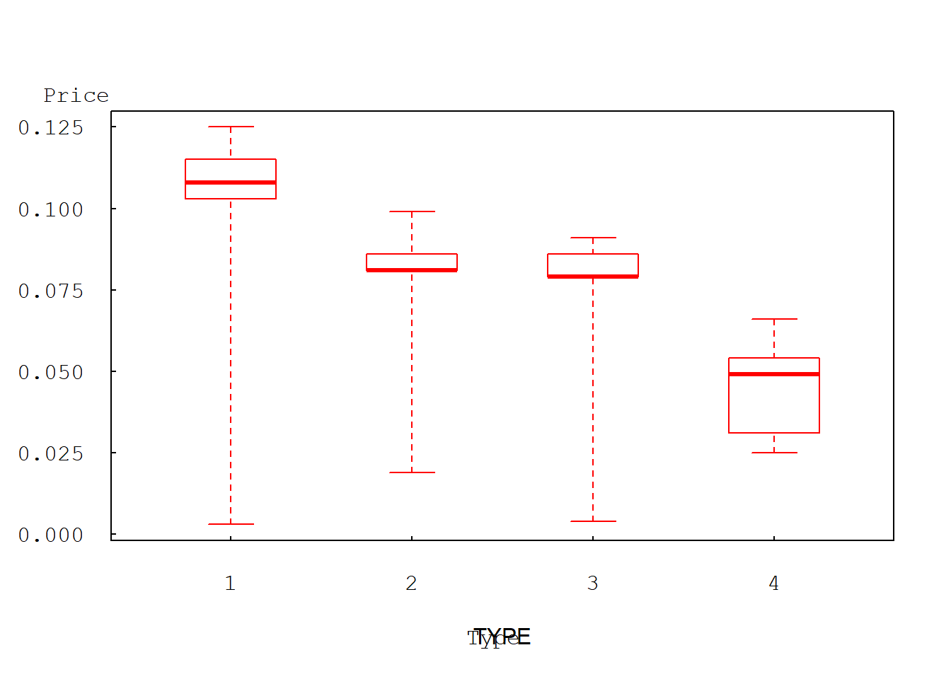
10.3.3 Note the small relationships among prices
cor(yogurtdata[, c("py", "pd", "pw", "ph")]) py pd pw ph
py 1.00000000 0.03201738 0.1538099 -0.01844819
pd 0.03201738 1.00000000 0.2428201 -0.04349290
pw 0.15380986 0.24282008 1.0000000 -0.02755800
ph -0.01844819 -0.04349290 -0.0275580 1.00000000plot(pw~pd, data=yogurtdata, yaxt="n", xaxt="n", ylab="", xlab="")
axis(2, at=seq(0.00, 0.20, by=0.01), las=1, font=10, cex=0.005, tck=0.01)
axis(2, at=seq(0.00, 0.20, by=0.002),lab=F, tck=0.005)
axis(1, at=seq(0.01, 0.12, by=0.01), font=10, cex=0.005, tck=0.01)
axis(1, at=seq(0.01, 0.12, by=0.002), lab=F, tck=0.005)
mtext("pw", side=2, line=1, at=0.11, las=1, font=10)
mtext("pd", side=1, line=3, at=0.062, font=10)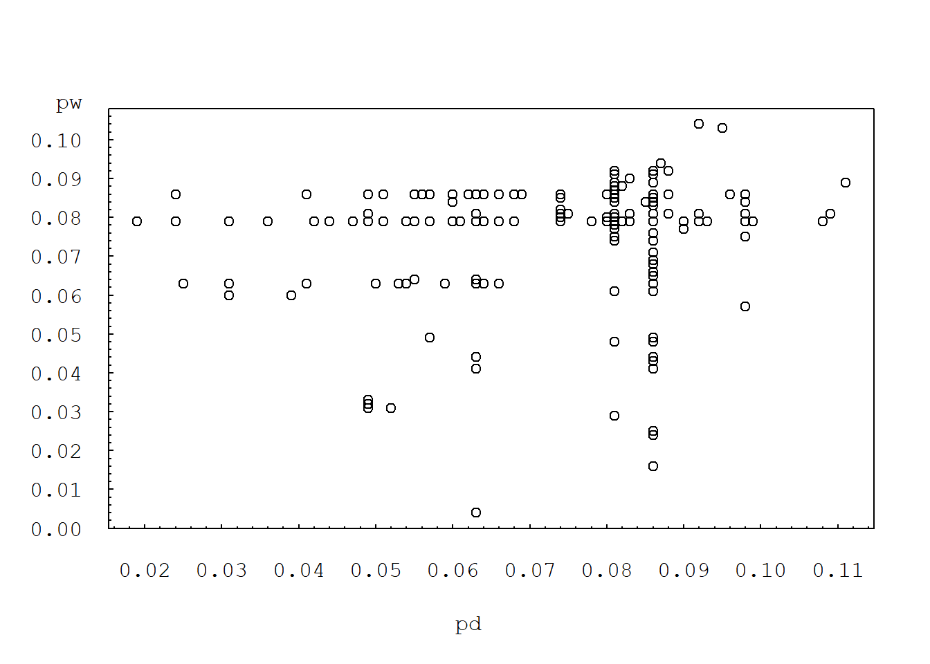
10.3.4 More on prices
summary(yogurtdata$PRICE) Min. 1st Qu. Median Mean 3rd Qu. Max.
0.00300 0.07900 0.08300 0.08495 0.10300 0.12500 range(yogurtdata$PRICE)[1] 0.003 0.125which(yogurtdata$PRICE == min(yogurtdata$PRICE))[1] 1210 1215 1930 1931 2381which(yogurtdata$PRICE == max(yogurtdata$PRICE))[1] 71 952 961 1212 1213 1214 1929 2199library(nnet)
test <- multinom(TYPE ~ FEATURE+PRICE, data = yogurtdata)# weights: 16 (9 variable)
initial value 3343.741999
iter 10 value 2587.908201
iter 20 value 2364.679552
iter 30 value 2360.691887
final value 2360.191855
convergedsummary(test)Call:
multinom(formula = TYPE ~ FEATURE + PRICE, data = yogurtdata)
Coefficients:
(Intercept) FEATURE PRICE
2 7.458657 -1.8039258 -80.44352
3 6.883787 -1.7072398 -80.32860
4 8.529886 -0.9595805 -139.53475
Std. Errors:
(Intercept) FEATURE PRICE
2 0.3509758 0.2400558 3.836776
3 0.3756930 0.2673651 4.169266
4 0.4773418 0.3787246 6.632942
Residual Deviance: 4720.384
AIC: 4738.384 10.4 Fitting fixed effects multinomial logit model by the poisson log-linear model
# RESHAPE yogurtdata FROM WIDE FORMAT INTO LONG FORMAT
yogurt<-reshape(yogurtdata, varying=list(c("yoplait","dannon","weight","hiland")), v.names=
"choice", idvar="occasion",timevar="brand", direction="long")
yogurt<-yogurt[order(yogurt$occasion),]
yogurt[1:8,]
id fy fd fw fh py pd pw ph occasion TYPE PRICE FEATURE
1.1 1 0 0 0 0 0.108 0.081 0.079 0.061 1 3 0.079 0
1.2 1 0 0 0 0 0.108 0.081 0.079 0.061 1 3 0.079 0
1.3 1 0 0 0 0 0.108 0.081 0.079 0.061 1 3 0.079 0
1.4 1 0 0 0 0 0.108 0.081 0.079 0.061 1 3 0.079 0
2.1 1 0 0 0 0 0.108 0.098 0.075 0.064 2 2 0.098 0
2.2 1 0 0 0 0 0.108 0.098 0.075 0.064 2 2 0.098 0
2.3 1 0 0 0 0 0.108 0.098 0.075 0.064 2 2 0.098 0
2.4 1 0 0 0 0 0.108 0.098 0.075 0.064 2 2 0.098 0
brand choice
1.1 1 0
1.2 2 0
1.3 3 1
1.4 4 0
2.1 1 0
2.2 2 1
2.3 3 0
2.4 4 0yogurt$brand<-factor(yogurt$brand)
yogurt$occasion<-factor(yogurt$occasion)
# yogurtloglinear<-glm(choice~brand+occasion+FEATURE+PRICE-1, data=yogurt, family=# poisson(link="log"))
# THE ABOVE GLM INCLUDES THE FIXED EFFECTS OF THE 2412 OCCASIONS, WHICH ARE
# NUISANCE PARAMETERS, THE ESTIMATES ARE NOT OBTAINED SIMPLY BECAUSE THE
# LARGE NUMBER.
# GLM USE ITERATIVELY REWEIGHTED LEAST SQUARES TO ESTIMATE, COMPARED WITH
# GENMOD IN SAS # USING MAXIMUMLIKELIHOOD.
# DROP occasion THE GLM IS ESTIMATABLE
model1 <- glm(choice~brand+FEATURE+PRICE-1, data=yogurt, family=poisson(link="log"))
summary(model1)
Call:
glm(formula = choice ~ brand + FEATURE + PRICE - 1, family = poisson(link = "log"),
    data = yogurt)

Deviance Residuals:
     Min        1Q    Median        3Q       Max
-0.89683  -0.82357  -0.67716   0.01585   2.26052

Coefficients:
          Estimate Std. Error z value Pr(>|z|)
brand1  -1.081e+00  9.183e-02  -11.78   <2e-16 ***
brand2  -9.109e-01  9.079e-02  -10.03   <2e-16 ***
brand3  -1.473e+00  9.497e-02  -15.51   <2e-16 ***
brand4  -3.526e+00  1.459e-01  -24.16   <2e-16 ***
FEATURE  3.206e-16  8.028e-02    0.00        1
PRICE   -1.375e-13  9.840e-01    0.00        1
---
Signif. codes:  0 '***' 0.001 '**' 0.01 '*' 0.05 '.' 0.1 ' ' 1

(Dispersion parameter for poisson family taken to be 1)

    Null deviance: 14472.0  on 9648  degrees of freedom
Residual deviance:  5665.9  on 9642  degrees of freedom
AIC: 10502

Number of Fisher Scoring iterations: 6
10.5 Fitting multinomial logit model with random intercepts by the possion-log-linear with random intercepts
library(MASS)
# glmmPQL(choice~feature+price+occasion, data=yogurt, family=poisson(link="log"), random=~1|brand)
# THE ABOVE HAS SIMILAR PROBLEM WHEN INCLUDING occasion AS FIXED EFFECTS
# OTHERWISE IT IS ESTIMATABLE IN R; HOWEVER THE RESULT IS QUITE DIFFERENT FROM # THAT OF SAS
glmmPQL(choice~FEATURE+PRICE, data=yogurt, family=poisson(link="log"), random=~1|brand)
iteration 1iteration 2iteration 3iteration 4iteration 5iteration 6Linear mixed-effects model fit by maximum likelihood
Data: yogurt
Log-likelihood: NA
Fixed: choice ~ FEATURE + PRICE
(Intercept) FEATURE PRICE
-1.743787e+00 2.005532e-14 2.982266e-13
Random effects:
Formula: ~1 | brand
(Intercept) Residual
StdDev: 1.040625 0.8639861
Variance function:
Structure: fixed weights
Formula: ~invwt
Number of Observations: 9648
Number of Groups: 4