Chapter 2 Fixed-Effects Models
2.1 Import Data
We consider T=6 years, 1990-1995, of data for inpatient hospital charges that are covered by the Medicare program. The data were obtained from the Health Care Financing Administration, Bureau of Data Management and Strategy. To illustrate, in 1995 the total covered charges were $157.8 billions for twelve million discharges. For this analysis, we use state as the subject, or risk class. Thus, we consider n=54 states that include the 50 states in the Union, the District of Columbia, Virgin Islands, Puerto Rico and an unspecified “other” category.
| Variable | Description |
|---|---|
| STATE | State identifier, 1-54 |
| YEAR | Year identifier, 1-6 |
| TOT_CHG | Total hospital charges, in millions of dollars. |
| COV_CHG | Total hospital charges covered by Medicare, in millions of dollars. |
| MED_REIM | Total hospital charges reimbursed by the Medicare program, in millions of dollars. |
| TOT_D | Total number of hospitals stays, in days. |
| NUM_DSHG | Number discharged, in thousands. |
| AVE_T_D | Average hospital stay per discharge in days. |
#  "\t"  INDICATES SEPARATED BY TABLES  ;
Medicare  = read.table("TXTData/Medicare.txt", sep ="\t", quote = "",header=TRUE)

# Medicare = read.table(choose.files(), sep ="\t", quote = "",header=TRUE)
Let’s have a look at the dataset. The names of variables and the first 8 rows observations.
#  PROVIDES THE NAMES IN THE FILE AND LISTS THE FIRST 8 OBSERVATIONS  ;
names (Medicare)
## [1] "STATE" "YEAR" "TOT_CHG" "COV_CHG" "MED_REIB" "TOT_D"
## [7] "NUM_DCHG" "AVE_T_D" "NMSTATE"Medicare [1:8, ]## STATE YEAR TOT_CHG COV_CHG MED_REIB TOT_D NUM_DCHG AVE_T_D
## 1 1 1 2211617271 2170240349 972752944 1932673 230015 8
## 2 1 2 2523987347 2468263759 1046016144 1936939 234739 8
## 3 1 3 2975969979 2922611694 1205791592 2016354 245027 8
## 4 1 4 3194595003 3149745611 1307982985 1948427 243947 8
## 5 1 5 3417704863 3384305357 1376211788 1926335 258384 7
## 6 1 6 3519375275 3492635576 1466220936 1847216 261738 7
## 7 2 1 64747759 62242279 42083051 51923 6636 8
## 8 2 2 70600503 67579913 46928596 53051 6940 8
## NMSTATE
## 1 AL
## 2 AL
## 3 AL
## 4 AL
## 5 AL
## 6 AL
## 7 AK
## 8 AKThen we need to create some other variables for later use.
#  CREATE OTHER VARIABLES;
# Firstly, we need change the names of existing variables.
names(Medicare)[names(Medicare)=="TOT_CHG"]="TOT.CHG";
names(Medicare)[names(Medicare)=="COV_CHG"]="COV.CHG";
names(Medicare)[names(Medicare)=="MED_REIB"]="MED.REIB";
names(Medicare)[names(Medicare)=="TOT_D"]="TOT.D";
names(Medicare)[names(Medicare)=="NUM_DCHG"]="NUM.DCHG";
names(Medicare)[names(Medicare)=="AVE_T_D"]="AVE.T.D";

Medicare$AVE.DAYS= Medicare$TOT.D/Medicare$NUM.DCHG
Medicare$CCPD=Medicare$COV.CHG/Medicare$NUM.DCHG
Medicare$NUM.DCHG=Medicare$NUM.DCHG/1000
str (Medicare)
## 'data.frame': 324 obs. of 11 variables:
## $ STATE : int 1 1 1 1 1 1 2 2 2 2 ...
## $ YEAR : int 1 2 3 4 5 6 1 2 3 4 ...
## $ TOT.CHG : num 2.21e+09 2.52e+09 2.98e+09 3.19e+09 3.42e+09 ...
## $ COV.CHG : num 2.17e+09 2.47e+09 2.92e+09 3.15e+09 3.38e+09 ...
## $ MED.REIB: num 9.73e+08 1.05e+09 1.21e+09 1.31e+09 1.38e+09 ...
## $ TOT.D : int 1932673 1936939 2016354 1948427 1926335 1847216 51923 53051 55191 53329 ...
## $ NUM.DCHG: num 230 235 245 244 258 ...
## $ AVE.T.D : int 8 8 8 8 7 7 8 8 7 7 ...
## $ NMSTATE : Factor w/ 54 levels "AK","AL","AR",..: 2 2 2 2 2 2 1 1 1 1 ...
## $ AVE.DAYS: num 8.4 8.25 8.23 7.99 7.46 ...
## $ CCPD : num 9435 10515 11928 12912 13098 ...Some summary statistics of CCPD, NUM.DCHG, AVE>DAYS, YEAR in each year.
library(nlme)
attach(Medicare)
#  SUMMARY STATISTICS ;
dim(Medicare)
## [1] 324 11summary(Medicare[, c("CCPD", "NUM.DCHG", "AVE.DAYS" )])## CCPD NUM.DCHG AVE.DAYS
## Min. : 2966 Min. : 0.515 Min. : 5.119
## 1st Qu.: 8537 1st Qu.: 42.715 1st Qu.: 7.162
## Median :10073 Median :144.282 Median : 8.067
## Mean :10483 Mean :210.731 Mean : 8.542
## 3rd Qu.:12059 3rd Qu.:282.884 3rd Qu.: 8.988
## Max. :21500 Max. :908.593 Max. :60.251gsummary(Medicare[, c("CCPD", "NUM.DCHG", "AVE.DAYS", "YEAR")], groups = YEAR, FUN=sd)## CCPD NUM.DCHG AVE.DAYS YEAR
## 1 2466.685 202.9918 2.077437 1
## 2 2711.568 210.3791 7.231312 2
## 3 3041.274 218.9225 1.858683 3
## 4 3259.846 219.8253 2.112467 4
## 5 3345.970 226.7783 1.728882 5
## 6 3277.985 229.4583 1.444423 6gsummary(Medicare[, c("CCPD", "NUM.DCHG", "AVE.DAYS", "YEAR")], groups = YEAR, FUN=mean)## CCPD NUM.DCHG AVE.DAYS YEAR
## 1 8503.168 197.7274 9.048565 1
## 2 9472.746 203.1443 9.823055 2
## 3 10443.285 210.8941 8.619240 3
## 4 11159.680 211.2479 8.522619 4
## 5 11522.826 218.8690 7.898816 5
## 6 11796.768 222.5059 7.342360 6gsummary(Medicare[, c("CCPD", "NUM.DCHG", "AVE.DAYS", "YEAR")], groups = YEAR, FUN=median)## CCPD NUM.DCHG AVE.DAYS YEAR
## 1 7991.927 142.5880 8.533565 1
## 2 9113.473 142.6935 8.570416 2
## 3 10055.416 143.2515 8.363435 3
## 4 10666.865 143.6720 8.112863 4
## 5 10955.142 150.0765 7.560945 5
## 6 11171.080 152.6960 7.143355 6gsummary(Medicare[, c("CCPD", "NUM.DCHG", "AVE.DAYS", "YEAR")], groups = YEAR, FUN=min)## CCPD NUM.DCHG AVE.DAYS YEAR
## 1 3228.989 0.528 6.326762 1
## 2 2966.117 0.515 6.143628 2
## 3 3324.113 0.653 5.830248 3
## 4 4137.776 0.969 5.830995 4
## 5 4354.526 1.156 5.378061 5
## 6 5058.371 1.059 5.118937 6gsummary(Medicare[, c("CCPD", "NUM.DCHG", "AVE.DAYS", "YEAR")], groups = YEAR, FUN=max)## CCPD NUM.DCHG AVE.DAYS YEAR
## 1 16484.77 849.372 17.47888 1
## 2 17636.51 885.919 60.25108 2
## 3 19814.09 908.593 16.35045 3
## 4 21121.55 894.216 17.13484 4
## 5 21500.29 905.615 14.38731 5
## 6 21031.58 902.479 12.79622 6See the box plots of different variables in each year.
#  ATTACH THE DATA SET FOR SOME PRELIMINARLY LOOKS;
attach (Medicare)
## The following objects are masked from Medicare (pos = 3):
##
## AVE.DAYS, AVE.T.D, CCPD, COV.CHG, MED.REIB, NMSTATE, NUM.DCHG,
## STATE, TOT.CHG, TOT.D, YEARMedicare$YEAR=Medicare$YEAR+1989
boxplot (CCPD ~ YEAR)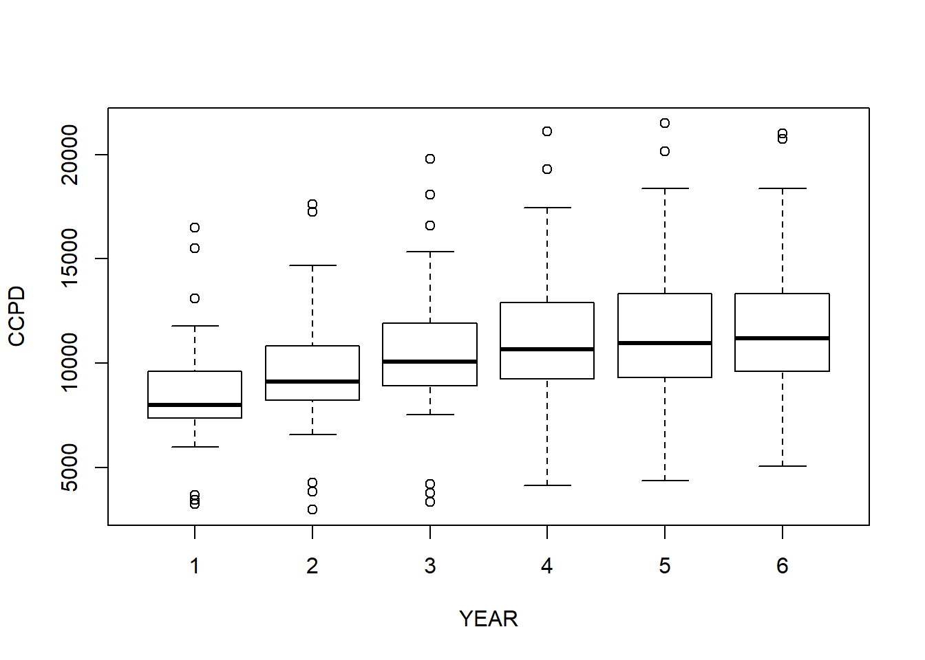
boxplot (NUM.DCHG ~ YEAR)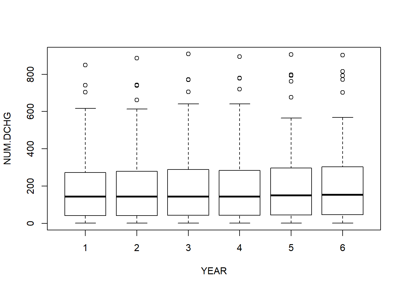
boxplot (AVE.DAYS ~ YEAR)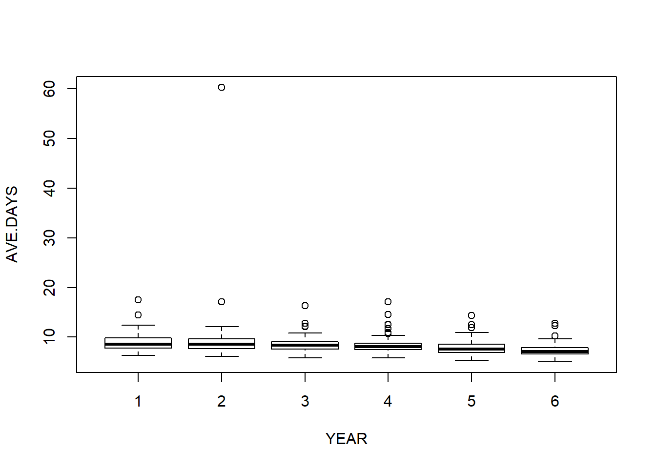
2.2 Example 2.2: Medicare Hospital Costs (Page 26)
2.2.1 FIGURE 2.1: CCPD vs YEAR; multiple time series plot
Figure 2.1 illustrates the multiple time-series plot. Here, we see that not only are overall claims increasing but also that claims increase for each state.
plot(CCPD ~ YEAR, data = Medicare, xaxt="n", yaxt="n", ylab="", xlab="")
 for (i in Medicare$STATE) {
 lines(CCPD ~ YEAR, data = subset(Medicare, STATE == i)) }
axis(2, at=seq(0, 22000, by=2000), las=1, font=10, cex=0.005, tck=0.01)
axis(1, at=seq(1990,1995, by=1), font=10, cex=0.005, tck=0.01)
mtext("CCPD", side=2, line=0, at=23000, font=12, cex=1, las=1)
mtext("YEAR", side=1, line=3, at=1992.5, font=12, cex=1)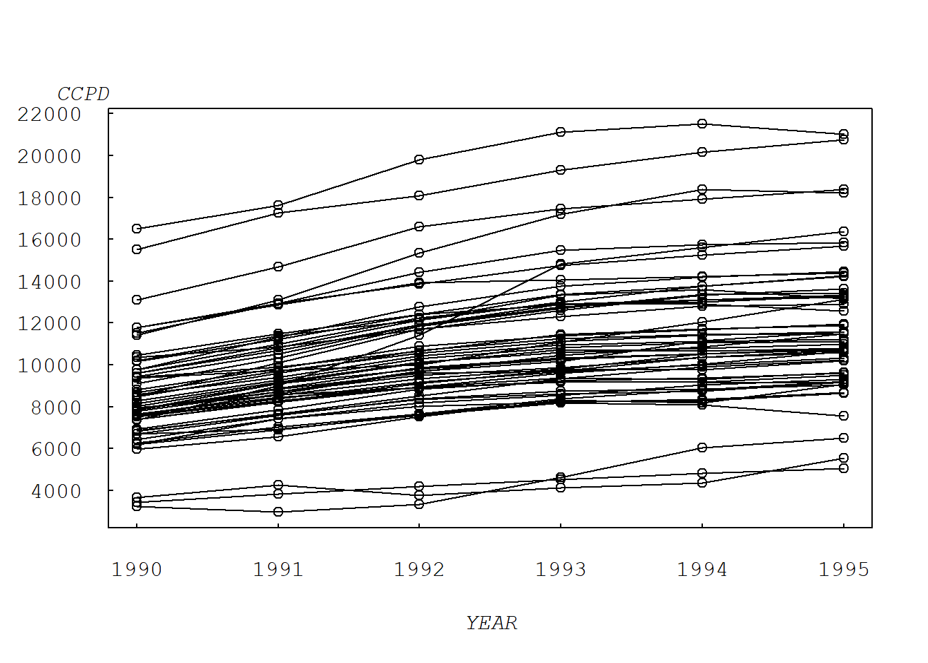
2.2.2 FIGURE 2.2: CCPD vs NUM.DCHG
Figure 2.2 illustrates the scatter plot with symbols. This plot ofCCPD versus number ofdischarges, connecting observations over time, shows a positive overall relationship between CCPD and the number of discharges.
plot(CCPD ~ NUM.DCHG, data = Medicare, xaxt="n", yaxt="n", ylab="", xlab="")
for (i in Medicare$STATE) {
 lines(CCPD ~ NUM.DCHG, data = subset(Medicare, STATE == i)) }
axis(2, at=seq(0, 22000, by=2000), las=1, font=10, cex=0.005, tck=0.01)
axis(2, at=seq(0, 22000, by=200), lab=F, tck=0.005)
axis(1, at=seq(0,1200, by=200), font=10, cex=0.005, tck=0.01)
axis(1, at=seq(0,1200, by=20), lab=F, tck=0.005)
mtext("CCPD", side=2, line=0, at=23000, font=12, cex=1, las=1)
mtext("Number of Discharges in Thousands", side=1, line=3, at=500, font=12, cex=1)
2.2.3 Figure 2.3: CCPD vs AVE.DAYS
Figure 2.3 is a scatter plot of CCPD versus average total days, connecting observations over time. This plot demonstrates the unusual nature of the second observation for the 54th state.
plot(CCPD ~ AVE.DAYS, data = Medicare, ylab="", xlab="", xaxt="n", yaxt="n")
for (i in Medicare$STATE) {
 lines(CCPD ~ AVE.DAYS, data = subset(Medicare, STATE== i)) }
axis(2, at=seq(0, 22000, by=2000), las=1, font=10, cex=0.005, tck=0.01)
axis(2, at=seq(0, 22000, by=200), lab=F, tck=0.005)
axis(1, at=seq(0,70, by=10), font=10, cex=0.005, tck=0.01)
axis(1, at=seq(0,70, by=1), lab=F, tck=0.005)
mtext("CCPD", side=2, line=0, at=23000, font=12, cex=1, las=1)
mtext("Average Hospital Stay", side=1, line=3, at=35, font=12, cex=1)
2.2.4 Figure 2.4: Added-variable plot of CCPD versus year
#  CREATE A CATEGORICAL VARIABLE for STATE;
Medicare$FSTATE = factor(Medicare$STATE)

#  CREATE A NEW VARIABLE;
Medicare$YEAR=Medicare$YEAR-1989
# THE NEW VARIABLES YR31 WILL BE USED IN THE FINAL MODEL TO GIVE THE 31st STATE A SPECIFIC SLOPE;
Medicare$Yr31=(Medicare$STATE==31)*Medicare$YEAR

#  CREATE A NEW DATA SET, REMOVING THE OUTLIER BY EXCLUDING THE 2ND OBSERVATION OF THE 54TH STATE;
Medicare2 = subset(Medicare, STATE != 54 | YEAR != 2)
Figure 2.4 illustrates the basic added-variable plot. This plot portrays CCPD versus year, after excluding the second observation for the 54th state.
#  BASIC ADDED VARIABLE PLOT;
#  CREATE RESIDUALS;
Med1.lm = lm(CCPD ~ FSTATE, data=Medicare2)
Med2.lm = lm(YEAR ~ FSTATE, data=Medicare2)
Medicare2$rCCPD=residuals(Med1.lm)
Medicare2$rYEAR=residuals(Med2.lm)
plot(rCCPD ~ rYEAR, data=Medicare2, ylab="", xlab="", xaxt="n", yaxt="n")
for (i in Medicare2$STATE) {
  lines(rCCPD ~ rYEAR, data = subset(Medicare2, STATE== i)) }
axis(2, at=seq(-6000, 4000, by=2000), las=1, font=10, cex=0.005, tck=0.01)
axis(2, at=seq(-6000, 4000, by=200), lab=F, tck=0.005)
axis(1, at=seq(-3,3, by=1), font=10, cex=0.005, tck=0.01)
axis(1, at=seq(-3,3, by=0.1), lab=F, tck=0.005)
mtext("Residuals from CCPD", side=2, line=-8, at=5000, font=12, cex=1, las=1)
mtext("Residuals from YEAR", side=1, line=3, at=0, font=12, cex=1)
2.2.5 Figure 2.5: Trellis Plot
A technique for graphical display that has recently become popular in the statistical literature is a trellis plot. This graphical technique takes its name from a trellis, which is a structure of open latticework. Figure 2.5 illustrates the use of small multiples. In each panel, the plot portrayed is identical except that it is based on a different state; this use of parallel structure allows us to demonstrate the increasing CCPD for each state.
GrpMedicare = groupedData(CCPD ~ YEAR| NMSTATE, data=Medicare2)
plot(GrpMedicare, xlab="YEAR", ylab="CCPD", scale = list(x=list(draw=FALSE)), layout=c(18,3))
2.3 One way fixed effects model using lm, for linear model
See Example 2.2: Medicare Hospital Costs.
Medicare.lm = lm(CCPD ~ NUM.DCHG + Yr31 + YEAR + AVE.DAYS + FSTATE - 1, data=Medicare2) # notice FSTATE is a factor variable created previously. Another way to fit a fixed effects model is :
Medicare.lm2 = lm(CCPD ~ NUM.DCHG + Yr31 + YEAR + AVE.DAYS + factor(STATE) - 1, data=Medicare2)

summary(Medicare.lm)
##
## Call:
## lm(formula = CCPD ~ NUM.DCHG + Yr31 + YEAR + AVE.DAYS + FSTATE -
## 1, data = Medicare2)
##
## Residuals:
## Min 1Q Median 3Q Max
## -1952.54 -264.66 50.46 300.10 1638.39
##
## Coefficients:
## Estimate Std. Error t value Pr(>|t|)
## NUM.DCHG 10.755 2.573 4.180 3.96e-05 ***
## Yr31 1262.456 128.609 9.816 < 2e-16 ***
## YEAR 710.884 26.812 26.513 < 2e-16 ***
## AVE.DAYS 361.290 57.979 6.231 1.81e-09 ***
## FSTATE1 3888.845 894.076 4.350 1.95e-05 ***
## FSTATE2 5694.017 534.048 10.662 < 2e-16 ***
## FSTATE3 5736.793 661.153 8.677 4.19e-16 ***
## FSTATE4 1639.697 726.577 2.257 0.02484 *
## FSTATE5 1745.883 2402.770 0.727 0.46810
## FSTATE6 5519.532 639.097 8.636 5.52e-16 ***
## FSTATE7 5882.663 815.649 7.212 5.77e-12 ***
## FSTATE8 6319.729 625.690 10.100 < 2e-16 ***
## FSTATE9 12842.939 733.122 17.518 < 2e-16 ***
## FSTATE10 990.386 1962.480 0.505 0.61422
## FSTATE11 1352.055 1020.337 1.325 0.18628
## FSTATE12 8524.447 790.980 10.777 < 2e-16 ***
## FSTATE13 2700.653 475.750 5.677 3.60e-08 ***
## FSTATE14 1417.162 1526.064 0.929 0.35392
## FSTATE15 1383.831 952.843 1.452 0.14760
## FSTATE16 1426.408 696.791 2.047 0.04163 *
## FSTATE17 3146.952 673.351 4.674 4.72e-06 ***
## FSTATE18 1728.006 844.017 2.047 0.04161 *
## FSTATE19 3926.979 867.993 4.524 9.16e-06 ***
## FSTATE20 3242.727 639.799 5.068 7.54e-07 ***
## FSTATE21 -711.562 898.191 -0.792 0.42894
## FSTATE22 1079.195 1161.922 0.929 0.35384
## FSTATE23 2480.023 1236.826 2.005 0.04596 *
## FSTATE24 2293.256 719.640 3.187 0.00161 **
## FSTATE25 957.334 712.831 1.343 0.18042
## FSTATE26 3299.585 998.712 3.304 0.00109 **
## FSTATE27 3003.060 494.942 6.068 4.47e-09 ***
## FSTATE28 3755.028 615.706 6.099 3.77e-09 ***
## FSTATE29 12615.456 598.073 21.094 < 2e-16 ***
## FSTATE30 4401.868 669.931 6.571 2.64e-10 ***
## FSTATE31 -2649.456 1345.138 -1.970 0.04992 *
## FSTATE32 3589.638 535.271 6.706 1.20e-10 ***
## FSTATE33 -4444.768 2367.411 -1.877 0.06155 .
## FSTATE34 1354.039 1071.140 1.264 0.20730
## FSTATE35 2683.031 552.483 4.856 2.05e-06 ***
## FSTATE36 -998.648 1578.677 -0.633 0.52755
## FSTATE37 2109.789 736.174 2.866 0.00449 **
## FSTATE38 3082.538 552.317 5.581 5.90e-08 ***
## FSTATE39 260.811 2145.305 0.122 0.90333
## FSTATE40 -2006.729 631.691 -3.177 0.00167 **
## FSTATE41 2978.161 744.200 4.002 8.16e-05 ***
## FSTATE42 3819.468 803.495 4.754 3.28e-06 ***
## FSTATE43 2398.622 532.257 4.507 9.90e-06 ***
## FSTATE44 1498.689 1017.547 1.473 0.14198
## FSTATE45 277.739 1831.029 0.152 0.87955
## FSTATE46 4580.418 496.141 9.232 < 2e-16 ***
## FSTATE47 3612.284 621.289 5.814 1.75e-08 ***
## FSTATE48 -2516.614 807.777 -3.115 0.00204 **
## FSTATE49 2213.600 943.221 2.347 0.01967 *
## FSTATE50 2138.158 685.695 3.118 0.00202 **
## FSTATE51 2101.881 677.712 3.101 0.00213 **
## FSTATE52 1138.089 835.624 1.362 0.17437
## FSTATE53 2784.381 471.058 5.911 1.04e-08 ***
## FSTATE54 -1037.318 544.265 -1.906 0.05774 .
## ---
## Signif. codes: 0 '***' 0.001 '**' 0.01 '*' 0.05 '.' 0.1 ' ' 1
##
## Residual standard error: 529.5 on 265 degrees of freedom
## Multiple R-squared: 0.9981, Adjusted R-squared: 0.9977
## F-statistic: 2392 on 58 and 265 DF, p-value: < 2.2e-16#summary(Medicare.lm2) # same as the summary(Medicare.lm)
anova(Medicare.lm)## Analysis of Variance Table
##
## Response: CCPD
## Df Sum Sq Mean Sq F value Pr(>F)
## NUM.DCHG 1 2.1693e+10 2.1693e+10 77387.47 < 2.2e-16 ***
## Yr31 1 6.8708e+07 6.8708e+07 245.11 < 2.2e-16 ***
## YEAR 1 1.1974e+10 1.1974e+10 42716.19 < 2.2e-16 ***
## AVE.DAYS 1 2.6659e+09 2.6659e+09 9510.30 < 2.2e-16 ***
## FSTATE 54 2.4833e+09 4.5986e+07 164.05 < 2.2e-16 ***
## Residuals 265 7.4284e+07 2.8032e+05
## ---
## Signif. codes: 0 '***' 0.001 '**' 0.01 '*' 0.05 '.' 0.1 ' ' 12.4 Section 2.4.1 - Analysis for the pooling test;
We can check the F-ratio by anova(Medicare.lm,Medicare3.lm). We reject the null hypothesis from the result below.
Medicare3.lm = lm(CCPD ~ NUM.DCHG+ Yr31 + YEAR + AVE.DAYS , data=Medicare2)
summary(Medicare3.lm)
##
## Call:
## lm(formula = CCPD ~ NUM.DCHG + Yr31 + YEAR + AVE.DAYS, data = Medicare2)
##
## Residuals:
## Min 1Q Median 3Q Max
## -7176.7 -1255.3 -384.9 1092.4 10350.9
##
## Coefficients:
## Estimate Std. Error t value Pr(>|t|)
## (Intercept) 4342.1049 873.4212 4.971 1.09e-06 ***
## NUM.DCHG 4.6606 0.7241 6.436 4.51e-10 ***
## Yr31 299.9270 295.8341 1.014 0.311432
## YEAR 733.2750 94.1398 7.789 9.62e-14 ***
## AVE.DAYS 308.4710 86.0766 3.584 0.000392 ***
## ---
## Signif. codes: 0 '***' 0.001 '**' 0.01 '*' 0.05 '.' 0.1 ' ' 1
##
## Residual standard error: 2732 on 318 degrees of freedom
## Multiple R-squared: 0.2879, Adjusted R-squared: 0.279
## F-statistic: 32.15 on 4 and 318 DF, p-value: < 2.2e-16anova(Medicare3.lm)## Analysis of Variance Table
##
## Response: CCPD
## Df Sum Sq Mean Sq F value Pr(>F)
## NUM.DCHG 1 463168764 463168764 62.0651 5.317e-14 ***
## Yr31 1 33908652 33908652 4.5438 0.0338046 *
## YEAR 1 366756374 366756374 49.1457 1.430e-11 ***
## AVE.DAYS 1 95840842 95840842 12.8428 0.0003919 ***
## Residuals 318 2373115933 7462629
## ---
## Signif. codes: 0 '***' 0.001 '**' 0.01 '*' 0.05 '.' 0.1 ' ' 1anova(Medicare3.lm,Medicare.lm) # pooling test## Analysis of Variance Table
##
## Model 1: CCPD ~ NUM.DCHG + Yr31 + YEAR + AVE.DAYS
## Model 2: CCPD ~ NUM.DCHG + Yr31 + YEAR + AVE.DAYS + FSTATE - 1
## Res.Df RSS Df Sum of Sq F Pr(>F)
## 1 318 2373115933
## 2 265 74284379 53 2298831554 154.73 < 2.2e-16 ***
## ---
## Signif. codes: 0 '***' 0.001 '**' 0.01 '*' 0.05 '.' 0.1 ' ' 1#F-statistic =154.73, reject the null hypothesis.2.5 Section 2.4.2 - Correlation corresponding to the added variable plot;
As with all scatter plots, the added-variable plot can be summarized numerically through a correlation coefficient that we will denote by \(corr(e_1, e_2)\).
#  Section 2.4.2 - CORRELATION CORRESPONDING TO THE ADDED VARIABLE PLOT;
library(boot)
cor(Medicare2$rCCPD , Medicare2$rYEAR)
## [1] 0.88471512.6 Section 2.4.5 - Testing for heteroscedasticity;
When fitting regression models to data, an important assumption is that the variability is common among all observations. This assumption of common variability is called homoscedasticity, meaning “same scatter”.
Medicare2$Resids=residuals(Medicare.lm)
Medicare2$ResidSq=Medicare2$Resids*Medicare2$Resids
MedHet.lm = lm(ResidSq ~ NUM.DCHG, data=Medicare2)
summary(MedHet.lm)
##
## Call:
## lm(formula = ResidSq ~ NUM.DCHG, data = Medicare2)
##
## Residuals:
## Min 1Q Median 3Q Max
## -255383 -212155 -143167 7752 3555249
##
## Coefficients:
## Estimate Std. Error t value Pr(>|t|)
## (Intercept) 261171.0 35324.5 7.393 1.25e-12 ***
## NUM.DCHG -147.5 116.8 -1.264 0.207
## ---
## Signif. codes: 0 '***' 0.001 '**' 0.01 '*' 0.05 '.' 0.1 ' ' 1
##
## Residual standard error: 454200 on 321 degrees of freedom
## Multiple R-squared: 0.004949, Adjusted R-squared: 0.001849
## F-statistic: 1.597 on 1 and 321 DF, p-value: 0.2073anova(MedHet.lm)## Analysis of Variance Table
##
## Response: ResidSq
## Df Sum Sq Mean Sq F value Pr(>F)
## NUM.DCHG 1 3.2930e+11 3.2930e+11 1.5966 0.2073
## Residuals 321 6.6208e+13 2.0625e+112.6.1 One way random effects model using lm, for linear model;
We will learn random effects model in Chapter 3. Here is an example. Here we provide two functions that can model random effects.
library(lme4)

Medicare.lme = lme(CCPD ~ NUM.DCHG, data=Medicare2, random = ~1|STATE) #lme()

Medicare.lmer=lmer(CCPD ~ NUM.DCHG+(1|STATE), data=Medicare2) #lmer()

summary(Medicare.lme)
## Linear mixed-effects model fit by REML
## Data: Medicare2
## AIC BIC logLik
## 5733.495 5748.581 -2862.747
##
## Random effects:
## Formula: ~1 | STATE
## (Intercept) Residual
## StdDev: 3016.201 1316.346
##
## Fixed effects: CCPD ~ NUM.DCHG
## Value Std.Error DF t-value p-value
## (Intercept) 8084.128 564.3211 268 14.325404 0
## NUM.DCHG 11.386 1.8044 268 6.310388 0
## Correlation:
## (Intr)
## NUM.DCHG -0.674
##
## Standardized Within-Group Residuals:
## Min Q1 Med Q3 Max
## -3.6167201 -0.6276783 0.1998388 0.6325460 2.7846480
##
## Number of Observations: 323
## Number of Groups: 54summary(Medicare.lmer)## Linear mixed model fit by REML ['lmerMod']
## Formula: CCPD ~ NUM.DCHG + (1 | STATE)
## Data: Medicare2
##
## REML criterion at convergence: 5725.5
##
## Scaled residuals:
## Min 1Q Median 3Q Max
## -3.6167 -0.6277 0.1998 0.6325 2.7846
##
## Random effects:
## Groups Name Variance Std.Dev.
## STATE (Intercept) 9097474 3016
## Residual 1732767 1316
## Number of obs: 323, groups: STATE, 54
##
## Fixed effects:
## Estimate Std. Error t value
## (Intercept) 8084.127 564.321 14.32
## NUM.DCHG 11.386 1.804 6.31
##
## Correlation of Fixed Effects:
## (Intr)
## NUM.DCHG -0.674#we can compare the results 2.7 More Fun
demo(graphics)##
##
## demo(graphics)
## ---- ~~~~~~~~
##
## > # Copyright (C) 1997-2009 The R Core Team
## >
## > require(datasets)
##
## > require(grDevices); require(graphics)
##
## > ## Here is some code which illustrates some of the differences between
## > ## R and S graphics capabilities. Note that colors are generally specified
## > ## by a character string name (taken from the X11 rgb.txt file) and that line
## > ## textures are given similarly. The parameter "bg" sets the background
## > ## parameter for the plot and there is also an "fg" parameter which sets
## > ## the foreground color.
## >
## >
## > x <- stats::rnorm(50)
##
## > opar <- par(bg = "white")
##
## > plot(x, ann = FALSE, type = "n")
##
## > abline(h = 0, col = gray(.90))
##
## > lines(x, col = "green4", lty = "dotted")
##
## > points(x, bg = "limegreen", pch = 21)
##
## > title(main = "Simple Use of Color In a Plot",
## +       xlab = "Just a Whisper of a Label",
## +       col.main = "blue", col.lab = gray(.8),
## +       cex.main = 1.2, cex.lab = 1.0, font.main = 4, font.lab = 3)
##
## > ## A little color wheel.    This code just plots equally spaced hues in
## > ## a pie chart.    If you have a cheap SVGA monitor (like me) you will
## > ## probably find that numerically equispaced does not mean visually
## > ## equispaced.  On my display at home, these colors tend to cluster at
## > ## the RGB primaries.  On the other hand on the SGI Indy at work the
## > ## effect is near perfect.
## >
## > par(bg = "gray")
##
## > pie(rep(1,24), col = rainbow(24), radius = 0.9)
##
## > title(main = "A Sample Color Wheel", cex.main = 1.4, font.main = 3)
##
## > title(xlab = "(Use this as a test of monitor linearity)",
## +       cex.lab = 0.8, font.lab = 3)
##
## > ## We have already confessed to having these.  This is just showing off X11
## > ## color names (and the example (from the postscript manual) is pretty "cute".
## >
## > pie.sales <- c(0.12, 0.3, 0.26, 0.16, 0.04, 0.12)
##
## > names(pie.sales) <- c("Blueberry", "Cherry",
## +              "Apple", "Boston Cream", "Other", "Vanilla Cream")
##
## > pie(pie.sales,
## +     col = c("purple","violetred1","green3","cornsilk","cyan","white"))
##
## > title(main = "January Pie Sales", cex.main = 1.8, font.main = 1)
##
## > title(xlab = "(Don't try this at home kids)", cex.lab = 0.8, font.lab = 3)
##
## > ## Boxplots:  I couldn't resist the capability for filling the "box".
## > ## The use of color seems like a useful addition, it focuses attention
## > ## on the central bulk of the data.
## >
## > par(bg="cornsilk")
##
## > n <- 10
##
## > g <- gl(n, 100, n*100)
##
## > x <- rnorm(n*100) + sqrt(as.numeric(g))
##
## > boxplot(split(x,g), col="lavender", notch=TRUE)
##
## > title(main="Notched Boxplots", xlab="Group", font.main=4, font.lab=1)
##
## > ## An example showing how to fill between curves.
## >
## > par(bg="white")
##
## > n <- 100
##
## > x <- c(0,cumsum(rnorm(n)))
##
## > y <- c(0,cumsum(rnorm(n)))
##
## > xx <- c(0:n, n:0)
##
## > yy <- c(x, rev(y))
##
## > plot(xx, yy, type="n", xlab="Time", ylab="Distance")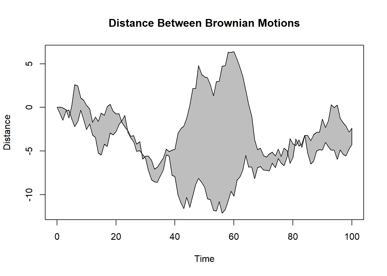
##
## > polygon(xx, yy, col="gray")
##
## > title("Distance Between Brownian Motions")
##
## > ## Colored plot margins, axis labels and titles.    You do need to be
## > ## careful with these kinds of effects.    It's easy to go completely
## > ## over the top and you can end up with your lunch all over the keyboard.
## > ## On the other hand, my market research clients love it.
## >
## > x <- c(0.00, 0.40, 0.86, 0.85, 0.69, 0.48, 0.54, 1.09, 1.11, 1.73, 2.05, 2.02)
##
## > par(bg="lightgray")
##
## > plot(x, type="n", axes=FALSE, ann=FALSE)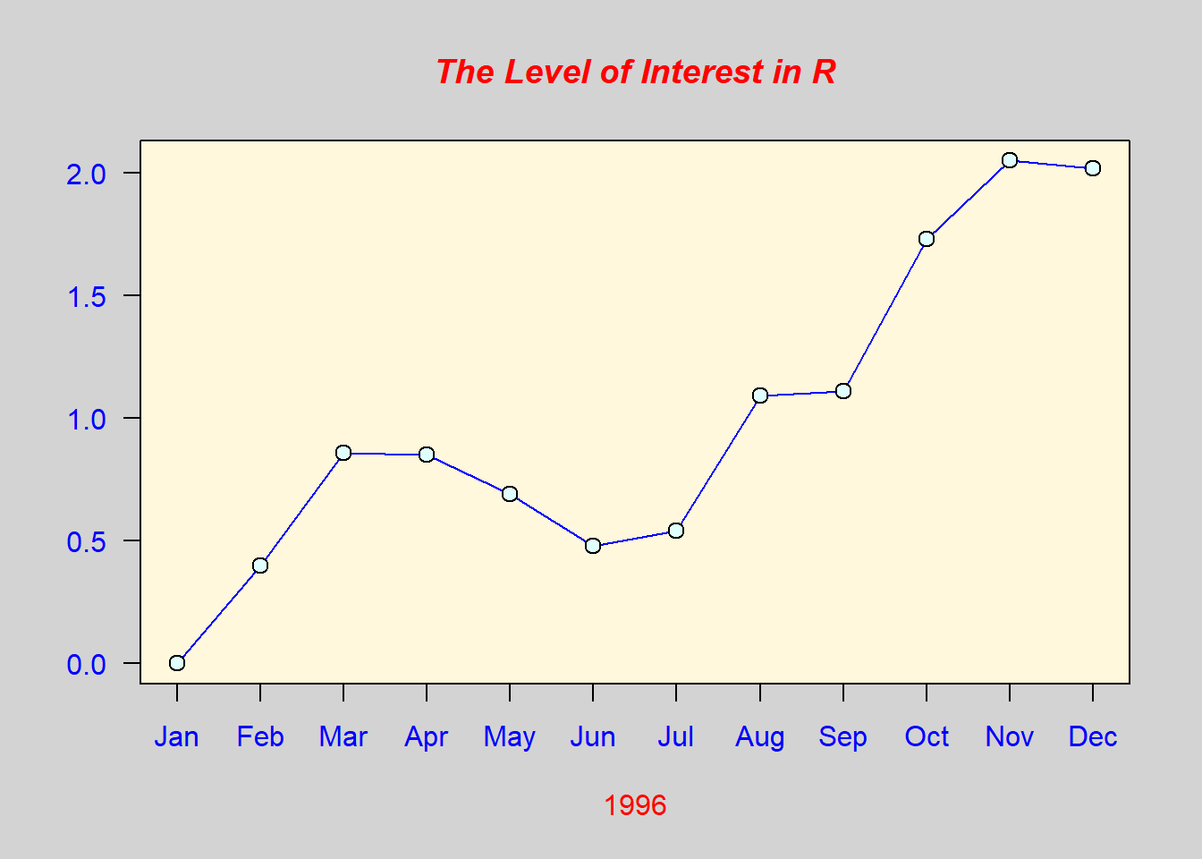
##
## > usr <- par("usr")
##
## > rect(usr[1], usr[3], usr[2], usr[4], col="cornsilk", border="black")
##
## > lines(x, col="blue")
##
## > points(x, pch=21, bg="lightcyan", cex=1.25)
##
## > axis(2, col.axis="blue", las=1)
##
## > axis(1, at=1:12, lab=month.abb, col.axis="blue")
##
## > box()
##
## > title(main= "The Level of Interest in R", font.main=4, col.main="red")
##
## > title(xlab= "1996", col.lab="red")
##
## > ## A filled histogram, showing how to change the font used for the
## > ## main title without changing the other annotation.
## >
## > par(bg="cornsilk")
##
## > x <- rnorm(1000)
##
## > hist(x, xlim=range(-4, 4, x), col="lavender", main="")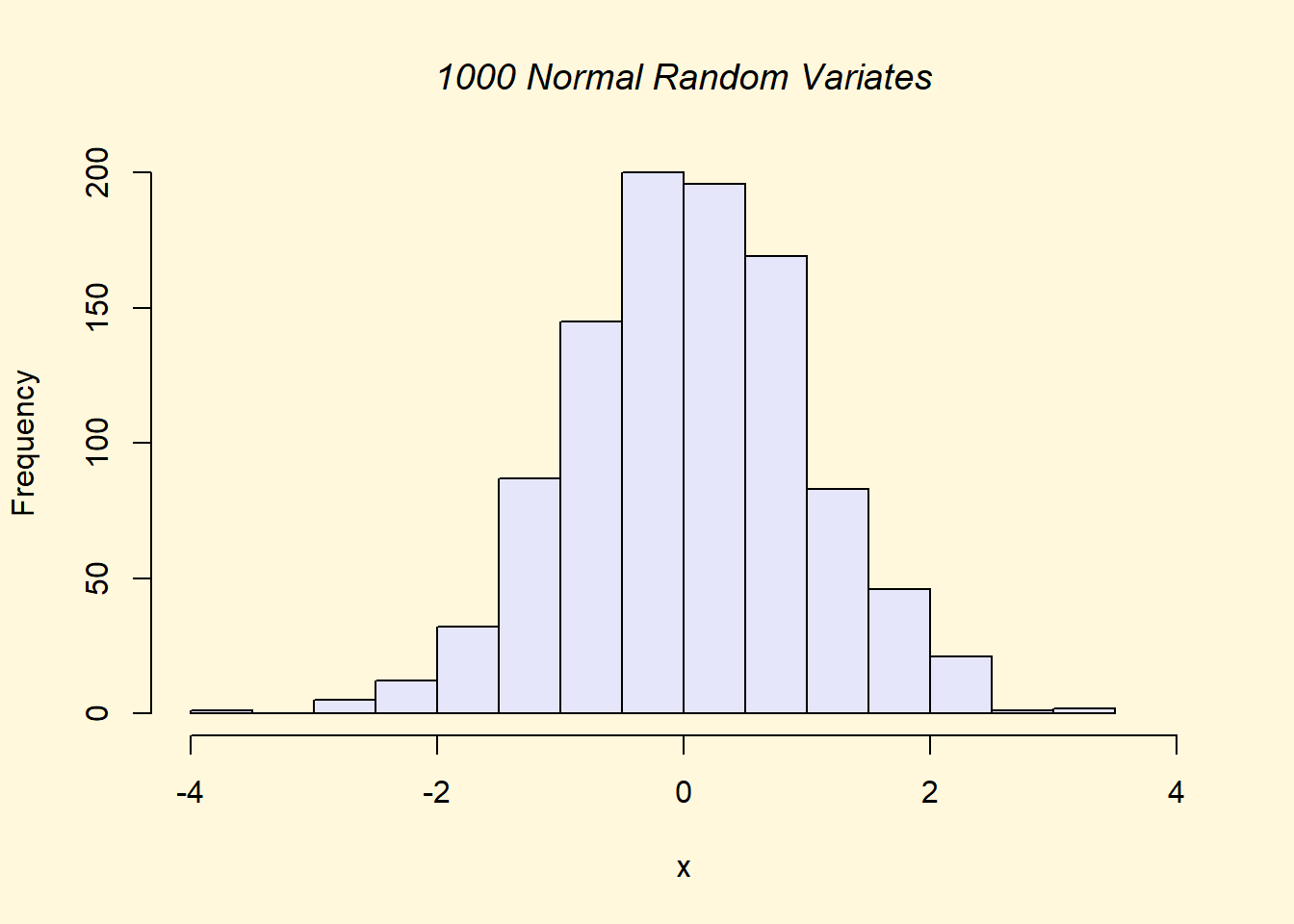
##
## > title(main="1000 Normal Random Variates", font.main=3)
##
## > ## A scatterplot matrix
## > ## The good old Iris data (yet again)
## >
## > pairs(iris[1:4], main="Edgar Anderson's Iris Data", font.main=4, pch=19)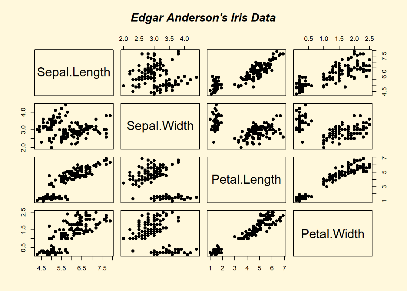
##
## > pairs(iris[1:4], main="Edgar Anderson's Iris Data", pch=21,
## +       bg = c("red", "green3", "blue")[unclass(iris$Species)])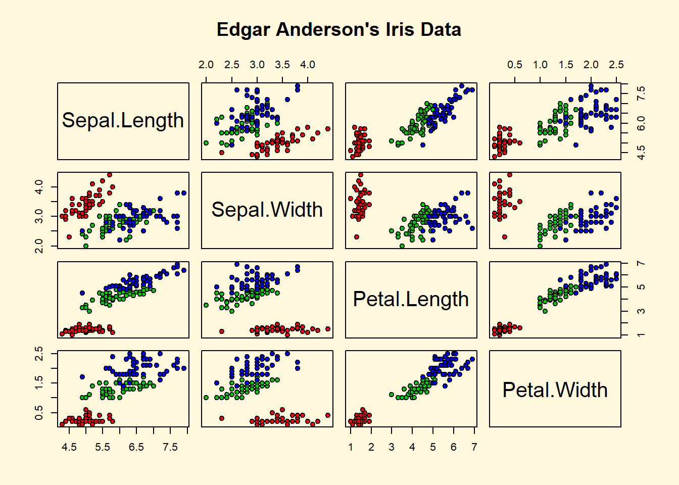
##
## > ## Contour plotting
## > ## This produces a topographic map of one of Auckland's many volcanic "peaks".
## >
## > x <- 10*1:nrow(volcano)
##
## > y <- 10*1:ncol(volcano)
##
## > lev <- pretty(range(volcano), 10)
##
## > par(bg = "lightcyan")
##
## > pin <- par("pin")
##
## > xdelta <- diff(range(x))
##
## > ydelta <- diff(range(y))
##
## > xscale <- pin[1]/xdelta
##
## > yscale <- pin[2]/ydelta
##
## > scale <- min(xscale, yscale)
##
## > xadd <- 0.5*(pin[1]/scale - xdelta)
##
## > yadd <- 0.5*(pin[2]/scale - ydelta)
##
## > plot(numeric(0), numeric(0),
## +      xlim = range(x)+c(-1,1)*xadd, ylim = range(y)+c(-1,1)*yadd,
## +      type = "n", ann = FALSE)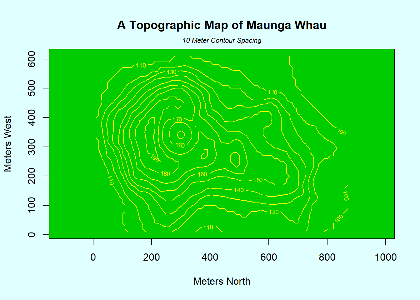
##
## > usr <- par("usr")
##
## > rect(usr[1], usr[3], usr[2], usr[4], col="green3")
##
## > contour(x, y, volcano, levels = lev, col="yellow", lty="solid", add=TRUE)
##
## > box()
##
## > title("A Topographic Map of Maunga Whau", font= 4)
##
## > title(xlab = "Meters North", ylab = "Meters West", font= 3)
##
## > mtext("10 Meter Contour Spacing", side=3, line=0.35, outer=FALSE,
## +       at = mean(par("usr")[1:2]), cex=0.7, font=3)
##
## > ## Conditioning plots
## >
## > par(bg="cornsilk")
##
## > coplot(lat ~ long | depth, data = quakes, pch = 21, bg = "green3")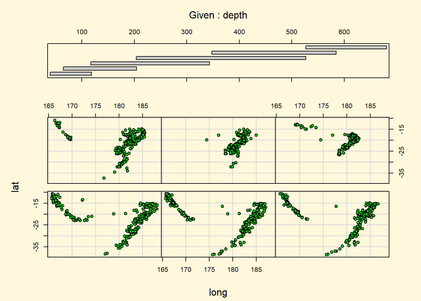
##
## > par(opar)
2.8 PLM (Panel Linear Model) package
library(plm)## Warning: package 'plm' was built under R version 3.6.1##
## Attaching package: 'plm'## The following object is masked from 'package:rmutil':
##
## nobsMedicarePool.plm <- plm(CCPD ~ NUM.DCHG + Yr31 + YEAR + AVE.DAYS, index=c("STATE","YEAR"),model="pooling",data=Medicare2)
summary(MedicarePool.plm)## Pooling Model
##
## Call:
## plm(formula = CCPD ~ NUM.DCHG + Yr31 + YEAR + AVE.DAYS, data = Medicare2,
## model = "pooling", index = c("STATE", "YEAR"))
##
## Unbalanced Panel: n = 54, T = 5-6, N = 323
##
## Residuals:
## Min. 1st Qu. Median 3rd Qu. Max.
## -7370.44 -1178.14 -442.63 1029.11 10201.10
##
## Coefficients:
## Estimate Std. Error t-value Pr(>|t|)
## (Intercept) 4878.45789 850.67127 5.7348 2.294e-08 ***
## NUM.DCHG 4.67811 0.72652 6.4391 4.501e-10 ***
## Yr31 307.06304 296.78045 1.0346 0.3016299
## YEAR2 1071.52446 530.17362 2.0211 0.0441195 *
## YEAR3 1994.97257 529.12820 3.7703 0.0001948 ***
## YEAR4 2732.79292 530.08887 5.1553 4.488e-07 ***
## YEAR5 3240.32483 538.72856 6.0148 5.007e-09 ***
## YEAR6 3657.24101 551.13882 6.6358 1.415e-10 ***
## AVE.DAYS 297.73052 86.73540 3.4326 0.0006779 ***
## ---
## Signif. codes: 0 '***' 0.001 '**' 0.01 '*' 0.05 '.' 0.1 ' ' 1
##
## Total Sum of Squares: 3332800000
## Residual Sum of Squares: 2357500000
## R-Squared: 0.29264
## Adj. R-Squared: 0.27462
## F-statistic: 16.2378 on 8 and 314 DF, p-value: < 2.22e-16MedicareFE.plm <- plm(CCPD ~ NUM.DCHG + Yr31 + YEAR + AVE.DAYS, index=c("STATE","YEAR"),model="within",data=Medicare2)
summary(MedicareFE.plm)## Oneway (individual) effect Within Model
##
## Call:
## plm(formula = CCPD ~ NUM.DCHG + Yr31 + YEAR + AVE.DAYS, data = Medicare2,
## model = "within", index = c("STATE", "YEAR"))
##
## Unbalanced Panel: n = 54, T = 5-6, N = 323
##
## Residuals:
## Min. 1st Qu. Median 3rd Qu. Max.
## -1957.51 -221.61 10.80 214.23 1686.75
##
## Coefficients:
## Estimate Std. Error t-value Pr(>|t|)
## NUM.DCHG 8.8577 2.3292 3.8029 0.0001781 ***
## Yr31 1265.7851 115.3637 10.9721 < 2.2e-16 ***
## YEAR2 921.0775 93.0311 9.9007 < 2.2e-16 ***
## YEAR3 1870.1890 97.6132 19.1592 < 2.2e-16 ***
## YEAR4 2581.0702 98.9237 26.0915 < 2.2e-16 ***
## YEAR5 2989.2386 115.8617 25.8000 < 2.2e-16 ***
## YEAR6 3328.8158 134.7499 24.7037 < 2.2e-16 ***
## AVE.DAYS 217.9681 55.0959 3.9562 9.82e-05 ***
## ---
## Signif. codes: 0 '***' 0.001 '**' 0.01 '*' 0.05 '.' 0.1 ' ' 1
##
## Total Sum of Squares: 538090000
## Residual Sum of Squares: 58858000
## R-Squared: 0.89062
## Adj. R-Squared: 0.86505
## F-statistic: 265.643 on 8 and 261 DF, p-value: < 2.22e-162.8.1 Pooling Test
pFtest(MedicareFE.plm,MedicarePool.plm)##
## F test for individual effects
##
## data: CCPD ~ NUM.DCHG + Yr31 + YEAR + AVE.DAYS
## F = 192.32, df1 = 53, df2 = 261, p-value < 2.2e-16
## alternative hypothesis: significant effects2.8.2 Two-way Model
MedicareTwoWay.plm <- plm(CCPD ~ NUM.DCHG + Yr31 + AVE.DAYS,
index=c("STATE","YEAR"),model="within",effect=c("twoways"),data=Medicare2)
summary(MedicareTwoWay.plm)## Twoways effects Within Model
##
## Call:
## plm(formula = CCPD ~ NUM.DCHG + Yr31 + AVE.DAYS, data = Medicare2,
## effect = c("twoways"), model = "within", index = c("STATE",
## "YEAR"))
##
## Unbalanced Panel: n = 54, T = 5-6, N = 323
##
## Residuals:
## Min. 1st Qu. Median 3rd Qu. Max.
## -1957.51 -221.61 10.80 214.23 1686.75
##
## Coefficients:
## Estimate Std. Error t-value Pr(>|t|)
## NUM.DCHG 8.8577 2.3292 3.8029 0.0001781 ***
## Yr31 1265.7851 115.3637 10.9721 < 2.2e-16 ***
## AVE.DAYS 217.9681 55.0959 3.9562 9.82e-05 ***
## ---
## Signif. codes: 0 '***' 0.001 '**' 0.01 '*' 0.05 '.' 0.1 ' ' 1
##
## Total Sum of Squares: 93740000
## Residual Sum of Squares: 58858000
## R-Squared: 0.37212
## Adj. R-Squared: 0.22538
## F-statistic: 51.5619 on 3 and 261 DF, p-value: < 2.22e-162.8.3 Three different ways to doing the same thing
MedicareFac.lm <- lm(CCPD ~ NUM.DCHG + Yr31 + factor(YEAR) + AVE.DAYS + FSTATE - 1, data=Medicare2)
summary(MedicareFac.lm)##
## Call:
## lm(formula = CCPD ~ NUM.DCHG + Yr31 + factor(YEAR) + AVE.DAYS +
## FSTATE - 1, data = Medicare2)
##
## Residuals:
## Min 1Q Median 3Q Max
## -1957.5 -221.6 10.8 214.2 1686.8
##
## Coefficients:
## Estimate Std. Error t value Pr(>|t|)
## NUM.DCHG 8.858 2.329 3.803 0.000178 ***
## Yr31 1265.785 115.364 10.972 < 2e-16 ***
## factor(YEAR)1 6026.365 817.464 7.372 2.22e-12 ***
## factor(YEAR)2 6947.442 819.299 8.480 1.69e-15 ***
## factor(YEAR)3 7896.554 824.936 9.572 < 2e-16 ***
## factor(YEAR)4 8607.435 821.760 10.474 < 2e-16 ***
## factor(YEAR)5 9015.603 813.052 11.089 < 2e-16 ***
## factor(YEAR)6 9355.180 800.204 11.691 < 2e-16 ***
## AVE.DAYS 217.968 55.096 3.956 9.82e-05 ***
## FSTATE2 1266.146 625.763 2.023 0.044055 *
## FSTATE3 1517.750 376.804 4.028 7.38e-05 ***
## FSTATE4 -2414.230 349.500 -6.908 3.75e-11 ***
## FSTATE5 -1043.426 1518.609 -0.687 0.492634
## FSTATE6 1320.333 425.863 3.100 0.002145 **
## FSTATE7 2125.483 379.338 5.603 5.34e-08 ***
## FSTATE8 2149.581 566.607 3.794 0.000184 ***
## FSTATE9 8956.546 546.207 16.398 < 2e-16 ***
## FSTATE10 -1988.208 1102.626 -1.803 0.072517 .
## FSTATE11 -2432.379 309.759 -7.852 1.06e-13 ***
## FSTATE12 4786.272 571.675 8.372 3.48e-15 ***
## FSTATE13 -1877.115 592.883 -3.166 0.001729 **
## FSTATE14 -1882.870 701.988 -2.682 0.007781 **
## FSTATE15 -2432.097 281.055 -8.653 5.22e-16 ***
## FSTATE16 -2695.687 363.328 -7.419 1.66e-12 ***
## FSTATE17 -983.973 398.410 -2.470 0.014161 *
## FSTATE18 -2183.247 283.342 -7.705 2.73e-13 ***
## FSTATE19 33.057 277.030 0.119 0.905110
## FSTATE20 -895.352 504.105 -1.776 0.076878 .
## FSTATE21 -4402.656 305.202 -14.425 < 2e-16 ***
## FSTATE22 -2294.496 374.263 -6.131 3.22e-09 ***
## FSTATE23 -1053.291 449.929 -2.341 0.019985 *
## FSTATE24 -1876.276 326.493 -5.747 2.53e-08 ***
## FSTATE25 -3138.855 351.389 -8.933 < 2e-16 ***
## FSTATE26 -453.848 294.614 -1.540 0.124654
## FSTATE27 -1521.817 575.983 -2.642 0.008736 **
## FSTATE28 -454.773 491.949 -0.924 0.356116
## FSTATE29 8371.800 539.053 15.531 < 2e-16 ***
## FSTATE30 349.923 537.126 0.651 0.515314
## FSTATE31 -5787.983 603.669 -9.588 < 2e-16 ***
## FSTATE32 -827.548 543.472 -1.523 0.129043
## FSTATE33 -6198.728 1418.515 -4.370 1.80e-05 ***
## FSTATE34 -2209.278 322.187 -6.857 5.07e-11 ***
## FSTATE35 -1682.747 562.379 -2.992 0.003035 **
## FSTATE36 -4288.776 753.597 -5.691 3.39e-08 ***
## FSTATE37 -1928.345 343.002 -5.622 4.84e-08 ***
## FSTATE38 -1371.812 456.168 -3.007 0.002894 **
## FSTATE39 -2428.130 1257.437 -1.931 0.054564 .
## FSTATE40 -6218.339 434.227 -14.320 < 2e-16 ***
## FSTATE41 -879.871 524.146 -1.679 0.094412 .
## FSTATE42 18.554 369.082 0.050 0.959945
## FSTATE43 -2022.863 562.920 -3.594 0.000390 ***
## FSTATE44 -2260.584 305.029 -7.411 1.74e-12 ***
## FSTATE45 -2801.199 981.990 -2.853 0.004684 **
## FSTATE46 58.371 572.520 0.102 0.918871
## FSTATE47 -572.015 581.201 -0.984 0.325932
## FSTATE48 -6229.345 632.766 -9.845 < 2e-16 ***
## FSTATE49 -1587.927 278.242 -5.707 3.12e-08 ***
## FSTATE50 -2077.178 349.181 -5.949 8.65e-09 ***
## FSTATE51 -2015.431 398.336 -5.060 7.93e-07 ***
## FSTATE52 -2853.564 280.020 -10.191 < 2e-16 ***
## FSTATE53 -1811.835 630.588 -2.873 0.004397 **
## FSTATE54 -5474.280 647.894 -8.449 2.08e-15 ***
## ---
## Signif. codes: 0 '***' 0.001 '**' 0.01 '*' 0.05 '.' 0.1 ' ' 1
##
## Residual standard error: 474.9 on 261 degrees of freedom
## Multiple R-squared: 0.9985, Adjusted R-squared: 0.9981
## F-statistic: 2782 on 62 and 261 DF, p-value: < 2.2e-16#str(summary(MedicareFac.lm))
MedicareFE.plm <- plm(CCPD ~ NUM.DCHG + Yr31 + YEAR + AVE.DAYS, index=c("STATE","YEAR"),model="within",data=Medicare2)
summary(MedicareFE.plm)
## Oneway (individual) effect Within Model
##
## Call:
## plm(formula = CCPD ~ NUM.DCHG + Yr31 + YEAR + AVE.DAYS, data = Medicare2,
## model = "within", index = c("STATE", "YEAR"))
##
## Unbalanced Panel: n = 54, T = 5-6, N = 323
##
## Residuals:
## Min. 1st Qu. Median 3rd Qu. Max.
## -1957.51 -221.61 10.80 214.23 1686.75
##
## Coefficients:
## Estimate Std. Error t-value Pr(>|t|)
## NUM.DCHG 8.8577 2.3292 3.8029 0.0001781 ***
## Yr31 1265.7851 115.3637 10.9721 < 2.2e-16 ***
## YEAR2 921.0775 93.0311 9.9007 < 2.2e-16 ***
## YEAR3 1870.1890 97.6132 19.1592 < 2.2e-16 ***
## YEAR4 2581.0702 98.9237 26.0915 < 2.2e-16 ***
## YEAR5 2989.2386 115.8617 25.8000 < 2.2e-16 ***
## YEAR6 3328.8158 134.7499 24.7037 < 2.2e-16 ***
## AVE.DAYS 217.9681 55.0959 3.9562 9.82e-05 ***
## ---
## Signif. codes: 0 '***' 0.001 '**' 0.01 '*' 0.05 '.' 0.1 ' ' 1
##
## Total Sum of Squares: 538090000
## Residual Sum of Squares: 58858000
## R-Squared: 0.89062
## Adj. R-Squared: 0.86505
## F-statistic: 265.643 on 8 and 261 DF, p-value: < 2.22e-16MedicareTwoWay.plm <- plm(CCPD ~ NUM.DCHG + Yr31 + AVE.DAYS,
index=c("STATE","YEAR"),model="within",effect=c("twoways"),data=Medicare2)
summary(MedicareTwoWay.plm)## Twoways effects Within Model
##
## Call:
## plm(formula = CCPD ~ NUM.DCHG + Yr31 + AVE.DAYS, data = Medicare2,
## effect = c("twoways"), model = "within", index = c("STATE",
## "YEAR"))
##
## Unbalanced Panel: n = 54, T = 5-6, N = 323
##
## Residuals:
## Min. 1st Qu. Median 3rd Qu. Max.
## -1957.51 -221.61 10.80 214.23 1686.75
##
## Coefficients:
## Estimate Std. Error t-value Pr(>|t|)
## NUM.DCHG 8.8577 2.3292 3.8029 0.0001781 ***
## Yr31 1265.7851 115.3637 10.9721 < 2.2e-16 ***
## AVE.DAYS 217.9681 55.0959 3.9562 9.82e-05 ***
## ---
## Signif. codes: 0 '***' 0.001 '**' 0.01 '*' 0.05 '.' 0.1 ' ' 1
##
## Total Sum of Squares: 93740000
## Residual Sum of Squares: 58858000
## R-Squared: 0.37212
## Adj. R-Squared: 0.22538
## F-statistic: 51.5619 on 3 and 261 DF, p-value: < 2.22e-162.8.4 Different r-squared - go figure
summary(MedicareFac.lm)$r.squared ## [1] 0.9984893summary(MedicareFE.plm)$r.squared ## rsq adjrsq
## 0.8906184 0.8650541summary(MedicareTwoWay.plm)$r.squared## rsq adjrsq
## 0.3721217 0.2253762