Chapter 4 Prediction and Bayesian Inference

4.1 Import Data

lottery  = read.table("TXTData/Lottery.txt", sep ="\t", quote = "",header=TRUE)

#lottery=read.table(choose.files(), header=TRUE, sep="\t")

State of Wisconsin lottery administrators provided weekly lottery sales data. We consider online lottery tickets that are sold by selected retail establishments in Wisconsin. These tickets are generally priced at $1.00, so the number of tickets sold equals the lottery revenue. We analyze lottery sales (OLSALES) over a forty-week period, April, 1998 through January, 1999, from fifty randomly selected ZIP codes within the state of Wisconsin. We also consider the number of retailers within a ZIP code for each time (NRETAIL).

Variable	Description
OLSALES	Online lottery sales to individual consumers
NRETAIL	Number of listed retailers
PERPERHH	Persons per household MEDSCHYR Median years of schooling
MEDHVL	Median home value in $1000s for owner-occupied homes PRCRENT
PRC55P	Percent of population that is 55 or older
HHMEDAGE	Household median age
MEDINC	Estimated median household income, in $1000s
POPULATN	Population, in thousands

#EXTRACT TIME - INVARIANT INFORMATION TO ANALYZE
mzip=d=as.data.frame(t(sapply(split(lottery[, c("NRETAIL", "PERPERHH", "OLSALES", "MEDSCHYR", "MEDHVL", "PRCRENT", "PRC55P", "HHMEDAGE", "MEDINC", "POPULATN")], lottery$ZIP),function(x) colMeans(x))))
 # Extract time invariant information to analyze
# Notice: the code for this part on website is wrong.

4.2 Example: Forecasting Wisconsin Lottery Sales (Page 138)

In this section, we forecast the sale of state lottery tickets from 50 postal (ZIP) codes inWisconsin. Lottery sales are an important component of state revenues. Accurate forecasting helps in the budget-planning process. A model is useful in assessing the important determinants of lottery sales, and understanding the determinants of lottery sales is useful for improving the design of the lottery sales system. Additional details of this study are in Frees and Miller (2003O).

4.2.1 TABLE 4.2: Time - invariant summary statistics

summary(mzip[,c("NRETAIL", "PERPERHH", "OLSALES", "MEDSCHYR", "MEDHVL", "PRCRENT", "PRC55P", "HHMEDAGE", "MEDINC", "POPULATN")]) 

##     NRETAIL          PERPERHH        OLSALES           MEDSCHYR    
##  Min.   : 1.000   Min.   :2.200   Min.   :  189.0   Min.   :12.20  
##  1st Qu.: 3.000   1st Qu.:2.600   1st Qu.:  821.3   1st Qu.:12.50  
##  Median : 6.362   Median :2.700   Median : 2426.4   Median :12.60  
##  Mean   :11.942   Mean   :2.706   Mean   : 6494.8   Mean   :12.70  
##  3rd Qu.:15.312   3rd Qu.:2.800   3rd Qu.:10016.5   3rd Qu.:12.78  
##  Max.   :68.625   Max.   :3.200   Max.   :33181.4   Max.   :15.90  
##      MEDHVL          PRCRENT          PRC55P        HHMEDAGE    
##  Min.   : 34.50   Min.   : 6.00   Min.   :25.0   Min.   :41.00  
##  1st Qu.: 43.77   1st Qu.:19.25   1st Qu.:35.0   1st Qu.:46.00  
##  Median : 53.90   Median :24.00   Median :40.0   Median :48.00  
##  Mean   : 57.09   Mean   :24.68   Mean   :39.7   Mean   :48.76  
##  3rd Qu.: 66.47   3rd Qu.:27.00   3rd Qu.:44.0   3rd Qu.:51.00  
##  Max.   :120.00   Max.   :62.00   Max.   :56.0   Max.   :59.00  
##      MEDINC         POPULATN     
##  Min.   :27.90   Min.   : 0.280  
##  1st Qu.:38.17   1st Qu.: 1.964  
##  Median :43.10   Median : 4.405  
##  Mean   :45.12   Mean   : 9.311  
##  3rd Qu.:53.62   3rd Qu.:15.446  
##  Max.   :70.70   Max.   :39.098

# STANDARD DEVIATION
sqrt(diag(var(mzip[,c("NRETAIL", "PERPERHH", "OLSALES", "MEDSCHYR", "MEDHVL", "PRCRENT", "PRC55P", "HHMEDAGE", "MEDINC", "POPULATN")]))) 

##      NRETAIL     PERPERHH      OLSALES     MEDSCHYR       MEDHVL 
##   13.2918231    0.2093820 8103.0125037    0.5514212   18.3731152 
##      PRCRENT       PRC55P     HHMEDAGE       MEDINC     POPULATN 
##    9.3425513    7.5112161    4.1431527    9.7835616   11.0981570

4.2.2 FIGURE 4.2: Look at the relationship

Figure 4.2 shows a positive relationship between average online sales and population. Further, the ZIP code corresponding to the city of Kenosha, Wisconsin, has unusually large average sales for its population size.

plot(OLSALES ~ POPULATN, data = mzip, xlab="", ylab="", xaxt="n", yaxt="n",pch="o", las=1, cex=1)

axis(2, at=seq(0, 40000, by=10000), las=1, font=10, cex=0.005, tck=0.01)

axis(2, at=seq(0, 40000, by=1000), lab=F, tck=0.005)

axis(1, at=seq(0,40, by=10), font=10, cex=0.005, tck=0.01)

axis(1, at=seq(0,40, by=1), lab=F, tck=0.005)

mtext("Average Lottery Sales", side=2, line=-3.5, at=36000, font=10, cex=1, las=1)

mtext("Population in Thousands", side=1, line=2, at=20, font=10, cex=1, las=1)

4.2.3 Sorting the data by zip then combine vectors into another data.frame

lottery$logsales<-log10(lottery$OLSALES)
m<-order(lottery$ZIP, lottery$TIME, lottery$OLSALES,lottery$logsales)

index<-as.data.frame(cbind(lottery$ZIP[m],lottery$TIME[m],lottery$OLSALES[m],lottery$logsales[m]))

names(index)<-c("ZIP", "TIME", "OLSALES", "LOGSALES")

4.2.4 FIGURE 4.3: Lottery vs. week number

Figure 4.3 presents a multiple time-series plot of (weekly) sales over time. Here, each line traces the sales patterns for a particular ZIP code. This figure shows the dramatic increase in sales for most ZIP codes, at approximately weeks 8 and 18.

plot(OLSALES ~ TIME, data = lottery, axes=F, ylab="", xlab="", xaxt="n", yaxt="n")
for (i in index$ZIP) {
     lines(OLSALES ~ TIME, data = subset(index, ZIP == i)) }
axis(1, at=seq(0,40, by=1), labels=F, tck=0.005)
axis(1, at=seq(0,40, by=10), cex=0.005, tck=0.01)
mtext("Week Number", side=1, line=2.5, cex=1, font=10)
axis(2, at=seq(0, 300000, by=10000), labels=F, tck=0.005)
axis(2, at=seq(0, 305000, by=100000), las=1, cex=0.005, tck=0.01) 
mtext("Lottery Sales", side=2, line=-3, at=310000, font=10, cex=1, las=1)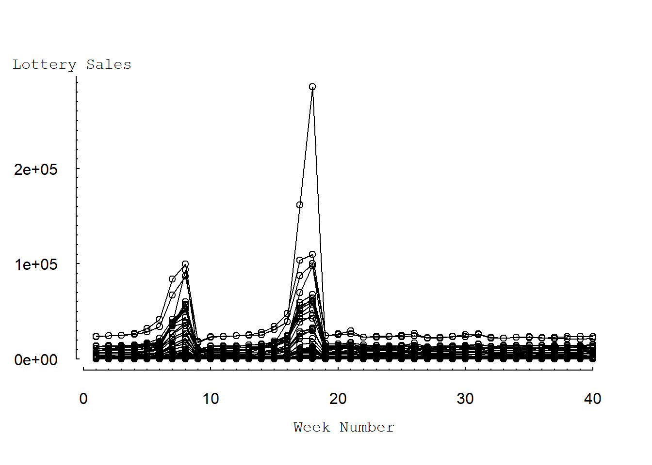

Another way of producing multiple time series graph by using trellis xyplot:

library(lattice)
trellis.device(color=F) # telling the trellis device to mimic 'black and white'
xyplot(OLSALES ~ TIME, data=index, groups=ZIP, scales=list(y=list(at=seq(0, 300000,100000), tck=.01)), panel=panel.superpose, pch=16, lty=1,  type="b")

#ChECK LOG VALUES
lottery$logsales<-log10(lottery$OLSALES)
lottery$lnsales<-log(lottery$OLSALES)

4.2.5 FIGURE 4.4: Log lottery vs week number

Figure 4.4 shows the same information as in Figure 4.3 but on a common (base 10) logarithmic scale. Here, we still see the effects of the PowerBall jackpots on sales. However, Figure 4.4 suggests a dynamic pattern that is common to all ZIP codes. Specifically, logarithmic sales for each ZIP code are relatively stable with the same approximate level of variability. Further, logarithmic sales for each ZIP code peak at the same time, corresponding to large PowerBall jackpots.

#FIGURE 4.4 LOG LOTTERY vs WEEK NUMBER
plot(LOGSALES ~ TIME, data = index, type="p", axes=F, ylab="", xlab="", pch=16, mkh=0.0001, lwd=0.5)
axis(1, at=seq(0,40, by=1), labels=F, tck=0.005)
axis(1, at=seq(0,40, by=10), cex=0.4, tck=0.01)
mtext("Week Number", side=1, line=2.5, cex=0.7, font=10)
axis(2, at=seq(0, 6, by=0.1), labels=F, tck=0.005)
axis(2, at=seq(0, 6, by=1), las=1, cex=0.4, tck=0.01) 
mtext("Logarithmic Lottery Sales", side=2, line=-1, at=5.8, font=10, cex=0.7, las=1)
    for (i in index$ZIP) {
    lines(LOGSALES ~ TIME, data=subset(index, ZIP==i)) }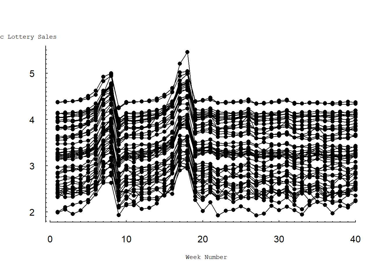

4.3 Create model development sample

Lottery=lottery
Lottery$LNSALES<-log(Lottery$OLSALES)
Lottery2<-subset(Lottery, Lottery$TIME<36)

4.3.1 MODEL 1. Pooled cross-setional model

lm1<-lm(LNSALES~PERPERHH+MEDSCHYR+MEDHVL+PRCRENT+PRC55P+HHMEDAGE+MEDINC+POPULATN+NRETAIL, data=Lottery2)
summary(lm1)#Pooled cross-sectional model 

## 
## Call:
## lm(formula = LNSALES ~ PERPERHH + MEDSCHYR + MEDHVL + PRCRENT + 
##     PRC55P + HHMEDAGE + MEDINC + POPULATN + NRETAIL, data = Lottery2)
## 
## Residuals:
##     Min      1Q  Median      3Q     Max 
## -1.9743 -0.6012 -0.0774  0.5430  4.2015 
## 
## Coefficients:
##              Estimate Std. Error t value Pr(>|t|)    
## (Intercept) 13.821060   1.339594  10.317  < 2e-16 ***
## PERPERHH    -1.084705   0.160224  -6.770 1.76e-11 ***
## MEDSCHYR    -0.821644   0.069049 -11.899  < 2e-16 ***
## MEDHVL       0.013822   0.002662   5.192 2.33e-07 ***
## PRCRENT      0.031820   0.003738   8.512  < 2e-16 ***
## PRC55P      -0.069578   0.013397  -5.194 2.30e-07 ***
## HHMEDAGE     0.118136   0.020961   5.636 2.03e-08 ***
## MEDINC       0.043373   0.005304   8.177 5.53e-16 ***
## POPULATN     0.057025   0.006060   9.410  < 2e-16 ***
## NRETAIL      0.021278   0.004076   5.220 2.00e-07 ***
## ---
## Signif. codes:  0 '***' 0.001 '**' 0.01 '*' 0.05 '.' 0.1 ' ' 1
## 
## Residual standard error: 0.8365 on 1740 degrees of freedom
## Multiple R-squared:  0.6963, Adjusted R-squared:  0.6947 
## F-statistic: 443.3 on 9 and 1740 DF,  p-value: < 2.2e-16

4.3.2 MODEL 2. Error components model

library(nlme)
lme1<-lme(LNSALES~PERPERHH+MEDSCHYR+MEDHVL+PRCRENT+PRC55P+HHMEDAGE+MEDINC+POPULATN+NRETAIL, data=Lottery2, random=~1|ZIP, method="REML") 
# NOTE* THE DEFAULT METHOD IN lme IS "REML"
# Use REML method in estimating fixed effects beta coefficients 
summary(lme1)

## Linear mixed-effects model fit by REML
##  Data: Lottery2 
##        AIC      BIC    logLik
##   2907.889 2973.428 -1441.944
## 
## Random effects:
##  Formula: ~1 | ZIP
##         (Intercept)  Residual
## StdDev:     0.77897 0.5130729
## 
## Fixed effects: LNSALES ~ PERPERHH + MEDSCHYR + MEDHVL + PRCRENT + PRC55P + HHMEDAGE +      MEDINC + POPULATN + NRETAIL 
##                 Value Std.Error   DF   t-value p-value
## (Intercept) 18.095695  7.316764 1699  2.473183  0.0135
## PERPERHH    -1.287021  0.886172   41 -1.452337  0.1540
## MEDSCHYR    -1.077937  0.375131   41 -2.873491  0.0064
## MEDHVL       0.007360  0.014633   41  0.502935  0.6177
## PRCRENT      0.026321  0.020660   41  1.274032  0.2098
## PRC55P      -0.072547  0.074259   41 -0.976939  0.3343
## HHMEDAGE     0.118637  0.116199   41  1.020986  0.3132
## MEDINC       0.045540  0.029396   41  1.549194  0.1290
## POPULATN     0.121851  0.027529   41  4.426231  0.0001
## NRETAIL     -0.027177  0.017420 1699 -1.560055  0.1189
##  Correlation: 
##          (Intr) PERPER MEDSCH MEDHVL PRCREN PRC55P HHMEDA MEDINC POPULA
## PERPERHH -0.632                                                        
## MEDSCHYR -0.745  0.204                                                 
## MEDHVL    0.303  0.093 -0.394                                          
## PRCRENT  -0.198  0.402 -0.258  0.008                                   
## PRC55P    0.146  0.236 -0.018  0.069  0.039                            
## HHMEDAGE -0.461  0.049  0.109 -0.128  0.151 -0.898                     
## MEDINC   -0.171 -0.013  0.080 -0.653  0.214  0.392 -0.200              
## POPULATN  0.180 -0.021 -0.228 -0.171 -0.287 -0.035  0.035 -0.050       
## NRETAIL  -0.210  0.082  0.246  0.159  0.096  0.014 -0.002 -0.027 -0.847
## 
## Standardized Within-Group Residuals:
##         Min          Q1         Med          Q3         Max 
## -2.06921597 -0.49881173 -0.29717361  0.02767368  6.60150830 
## 
## Number of Observations: 1750
## Number of Groups: 50

# CHECK AUTOCORRELATION PATTERNS
ACF(lme1, maxlag=10) #Obtain ACF of residuals from lme1

##    lag         ACF
## 1    0  1.00000000
## 2    1  0.52724776
## 3    2  0.10000857
## 4    3 -0.03788895
## 5    4 -0.15969734
## 6    5 -0.23410399
## 7    6 -0.24984691
## 8    7 -0.18355756
## 9    8 -0.02825433
## 10   9  0.19456638
## 11  10  0.47143962
## 12  11  0.17601528
## 13  12 -0.10862546
## 14  13 -0.16449717
## 15  14 -0.31225995
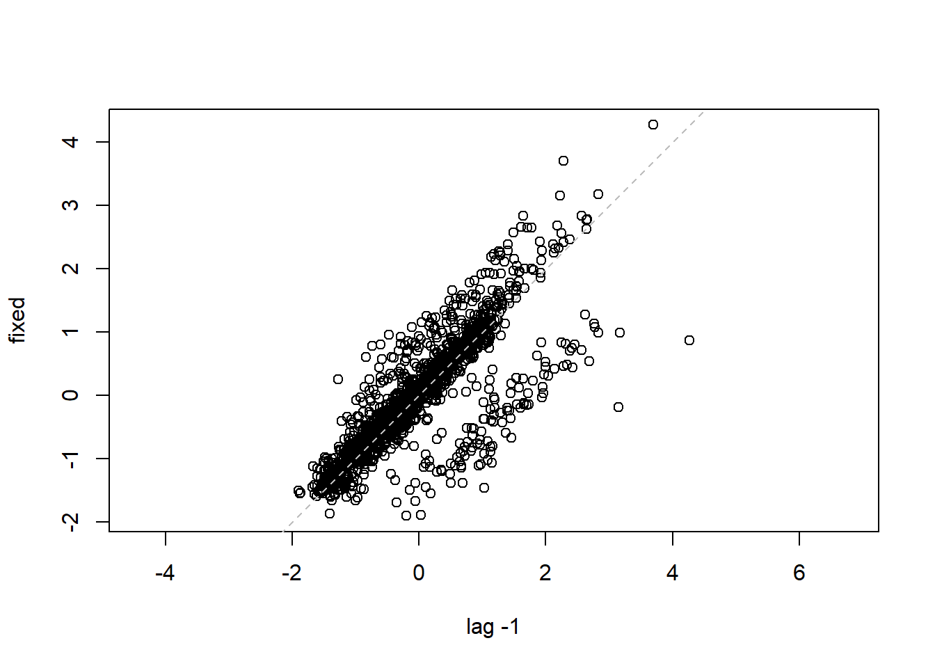
## 16  15 -0.40819498

lag.plot(lme1$residuals, lags=-1) #Autocorrelation patterns one lag, needs to refine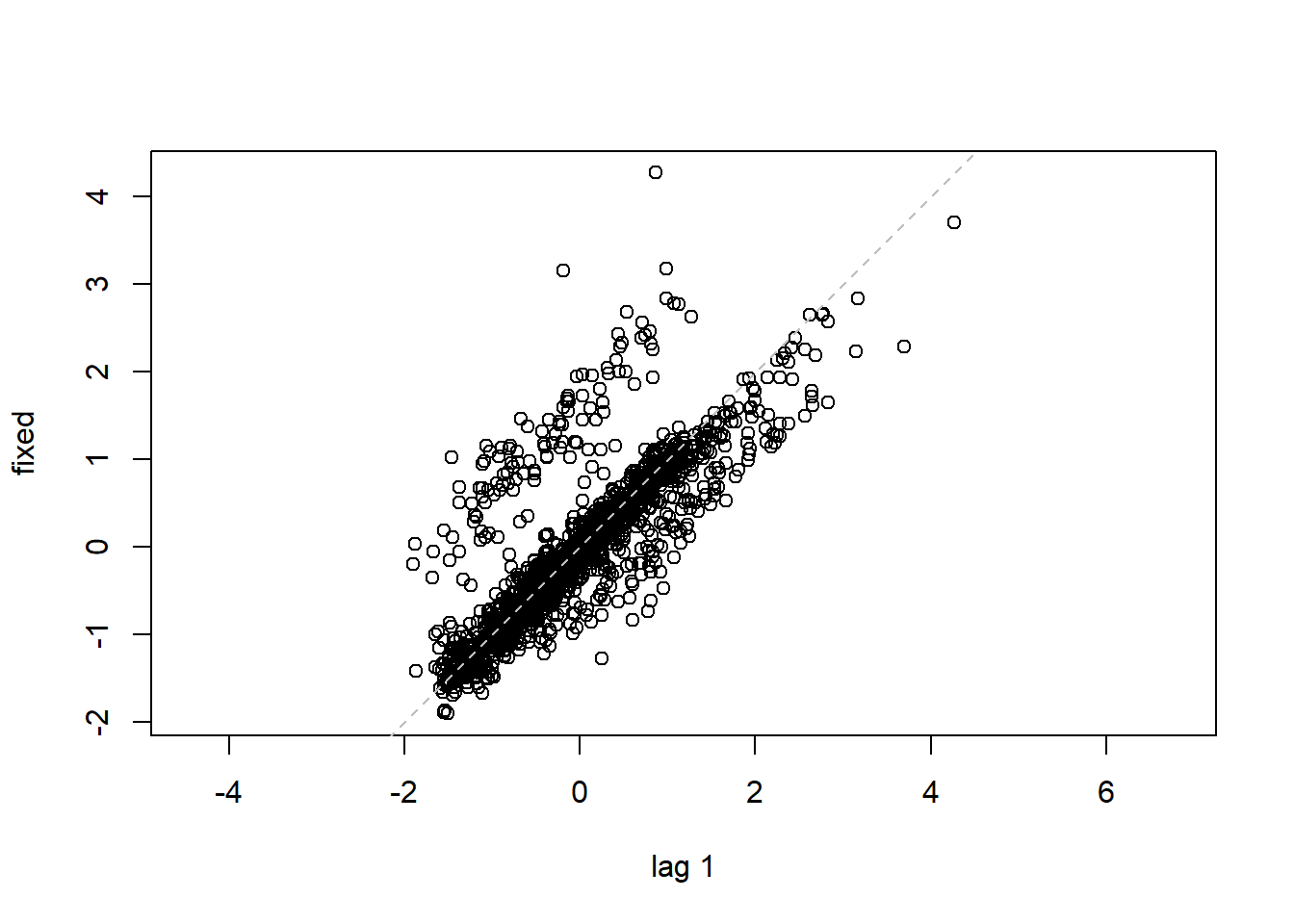

4.3.3 MODEL 3. Error components model with autocorrelated errors

lme2<-update(lme1, correlation=corAR1(form=~TIME|ZIP))
summary(lme2)

## Linear mixed-effects model fit by REML
##  Data: Lottery2 
##        AIC      BIC    logLik
##   2318.834 2389.835 -1146.417
## 
## Random effects:
##  Formula: ~1 | ZIP
##         (Intercept)  Residual
## StdDev:    0.726541 0.5282642
## 
## Correlation Structure: AR(1)
##  Formula: ~TIME | ZIP 
##  Parameter estimate(s):
##       Phi 
## 0.5552575 
## Fixed effects: LNSALES ~ PERPERHH + MEDSCHYR + MEDHVL + PRCRENT + PRC55P + HHMEDAGE +      MEDINC + POPULATN + NRETAIL 
##                 Value Std.Error   DF    t-value p-value
## (Intercept) 15.254535  7.005477 1699  2.1775157  0.0296
## PERPERHH    -1.149312  0.842554   41 -1.3640808  0.1800
## MEDSCHYR    -0.911242  0.360225   41 -2.5296504  0.0154
## MEDHVL       0.011273  0.013960   41  0.8074825  0.4240
## PRCRENT      0.030104  0.019652   41  1.5319015  0.1332
## PRC55P      -0.071434  0.070515   41 -1.0130333  0.3170
## HHMEDAGE     0.119779  0.110336   41  1.0855851  0.2840
## MEDINC       0.044082  0.027916   41  1.5790867  0.1220
## POPULATN     0.080430  0.029449   41  2.7311900  0.0093
## NRETAIL      0.003887  0.019402 1699  0.2003424  0.8412
##  Correlation: 
##          (Intr) PERPER MEDSCH MEDHVL PRCREN PRC55P HHMEDA MEDINC POPULA
## PERPERHH -0.632                                                        
## MEDSCHYR -0.750  0.209                                                 
## MEDHVL    0.286  0.097 -0.373                                          
## PRCRENT  -0.204  0.403 -0.246  0.014                                   
## PRC55P    0.144  0.236 -0.017  0.069  0.039                            
## HHMEDAGE -0.457  0.049  0.108 -0.128  0.151 -0.898                     
## MEDINC   -0.167 -0.014  0.077 -0.652  0.212  0.392 -0.200              
## POPULATN  0.217 -0.042 -0.269 -0.196 -0.281 -0.035  0.032 -0.037       
## NRETAIL  -0.245  0.097  0.285  0.185  0.112  0.017 -0.002 -0.031 -0.881
## 
## Standardized Within-Group Residuals:
##         Min          Q1         Med          Q3         Max 
## -1.87105785 -0.46121477 -0.26278521  0.04905521  6.55032232 
## 
## Number of Observations: 1750
## Number of Groups: 50

4.3.4 MODEL 4. More parsimonious random effects model

With fewer covariates:

lme3<-lme(LNSALES~MEDSCHYR+POPULATN, data=Lottery2, random=~1|ZIP, correlation=corAR1(form=~TIME|ZIP))

#The pooled cross-sectional model with autocorrelated errors
#Default method for gls is reml, gls can be viewed as an lme function without the argument random
library(nlme)
gls1<-gls(LNSALES~PERPERHH+MEDSCHYR+MEDHVL+PRCRENT+PRC55P+HHMEDAGE+MEDINC+POPULATN+NRETAIL, data=Lottery2, correlation=corAR1(form=~TIME|ZIP)) 
summary(gls1)

## Generalized least squares fit by REML
##   Model: LNSALES ~ PERPERHH + MEDSCHYR + MEDHVL + PRCRENT + PRC55P + HHMEDAGE +      MEDINC + POPULATN + NRETAIL 
##   Data: Lottery2 
##        AIC      BIC    logLik
##   2505.647 2571.186 -1240.823
## 
## Correlation Structure: AR(1)
##  Formula: ~TIME | ZIP 
##  Parameter estimate(s):
##       Phi 
## 0.8240088 
## 
## Coefficients:
##                 Value Std.Error   t-value p-value
## (Intercept) 13.596133  3.858304  3.523863  0.0004
## PERPERHH    -1.063225  0.461639 -2.303151  0.0214
## MEDSCHYR    -0.820030  0.198788 -4.125146  0.0000
## MEDHVL       0.012934  0.007667  1.686984  0.0918
## PRCRENT      0.032524  0.010771  3.019630  0.0026
## PRC55P      -0.072183  0.038596 -1.870207  0.0616
## HHMEDAGE     0.122852  0.060391  2.034284  0.0421
## MEDINC       0.043223  0.015281  2.828636  0.0047
## POPULATN     0.058989  0.017339  3.402168  0.0007
## NRETAIL      0.020143  0.011647  1.729449  0.0839
## 
##  Correlation: 
##          (Intr) PERPER MEDSCH MEDHVL PRCREN PRC55P HHMEDA MEDINC POPULA
## PERPERHH -0.633                                                        
## MEDSCHYR -0.754  0.213                                                 
## MEDHVL    0.275  0.101 -0.359                                          
## PRCRENT  -0.208  0.405 -0.237  0.018                                   
## PRC55P    0.142  0.237 -0.016  0.069  0.039                            
## HHMEDAGE -0.454  0.049  0.107 -0.127  0.151 -0.898                     
## MEDINC   -0.165 -0.014  0.075 -0.651  0.211  0.392 -0.200              
## POPULATN  0.242 -0.056 -0.295 -0.212 -0.280 -0.035  0.029 -0.030       
## NRETAIL  -0.267  0.107  0.310  0.202  0.124  0.018 -0.001 -0.033 -0.898
## 
## Standardized residuals:
##         Min          Q1         Med          Q3         Max 
## -2.26140351 -0.64050416 -0.02884818  0.69976712  5.08212114 
## 
## Residual standard error: 0.8427768 
## Degrees of freedom: 1750 total; 1740 residual

#getVarCov(gls1)
anova(gls1,lm1)

##      Model df      AIC      BIC    logLik   Test  L.Ratio p-value
## gls1     1 12 2505.647 2571.186 -1240.823                        
## lm1      2 11 4430.126 4490.204 -2204.063 1 vs 2 1926.479  <.0001

#using anova for the models with serial correlation and the pooled cross–sectional regression.

4.3.5 MODEL 5. Fixed effects model with autocorrelated errors

Lottery2$ZIPfac=factor(Lottery2$ZIP)
gls2<-gls(LNSALES~ZIPfac, data=Lottery2, correlation=corAR1(form=~TIME|ZIPfac)) 
gls2

## Generalized least squares fit by REML
##   Model: LNSALES ~ ZIPfac 
##   Data: Lottery2 
##   Log-restricted-likelihood: -1073.063
## 
## Coefficients:
## (Intercept) ZIPfac53033 ZIPfac53038 ZIPfac53059 ZIPfac53072 ZIPfac53083 
##  7.02034302  1.07644720  0.61877604 -0.01329196  2.45963633  1.97648544 
## ZIPfac53095 ZIPfac53098 ZIPfac53104 ZIPfac53172 ZIPfac53211 ZIPfac53520 
##  3.27341024  0.59051473  2.12004892  2.56764964  2.68989060  1.53954270 
## ZIPfac53544 ZIPfac53563 ZIPfac53572 ZIPfac53574 ZIPfac53813 ZIPfac53924 
## -1.22340317  1.68388653  0.81336415  0.64605315  0.79960910 -1.46385511 
## ZIPfac53934 ZIPfac53943 ZIPfac53952 ZIPfac54115 ZIPfac54143 ZIPfac54153 
##  0.65471544 -1.31041280  0.49735851  2.03324306  2.40463509  1.12075652 
## ZIPfac54170 ZIPfac54205 ZIPfac54213 ZIPfac54220 ZIPfac54235 ZIPfac54241 
## -0.09585752 -0.80190426 -0.69482488  3.22278219  2.21634671  1.96067334 
## ZIPfac54302 ZIPfac54406 ZIPfac54436 ZIPfac54457 ZIPfac54470 ZIPfac54474 
##  2.39541360  0.75120386 -1.31334267  1.60733345 -0.28003078  0.51088577 
## ZIPfac54480 ZIPfac54531 ZIPfac54556 ZIPfac54614 ZIPfac54622 ZIPfac54634 
## -1.62581025 -0.73327749 -0.37613230 -0.50434660 -0.79801244  0.49941189 
## ZIPfac54650 ZIPfac54701 ZIPfac54724 ZIPfac54745 ZIPfac54758 ZIPfac54810 
##  2.50724987  2.72121016  0.66159018 -0.99678783  0.71914194 -1.16821041 
## ZIPfac54839 ZIPfac54956 
## -2.00207902  2.57602144 
## 
## Correlation Structure: AR(1)
##  Formula: ~TIME | ZIPfac 
##  Parameter estimate(s):
##     Phi 
## 0.55476 
## Degrees of freedom: 1750 total; 1700 residual
## Residual standard error: 0.5279669

#getVarCov(gls2) # Show the covariance matrix, the AR(1) structure

# Note the difference between R estimates and SAS estimates is because in SAS the estimate 
# for ZIP 54956 is restricted to be zero, in R the intercept and estimates for Zip are 
# scaled differently, but both estimates should give us approximately the same answer#

The five models listed are summarized in Table 4.4 at Page 146.