Chapter 5 Multilevel Models
5.1 Import Data
#Dental=read.table(choose.files(), header=TRUE, sep="\t")
#library(mice)
#data(potthoffroy)
# I make this dataset myself according to data(potthoffroy)
Dental <- read.table("TXTData/dental.txt",sep ="\t", quote = "", header=TRUE)

names(Dental)<-c("MEASURE", "SEX", "AGE", "ID")
5.2 Example 5.2: Dental Data (Page 175)
This example is originally due to Potthoff and Roy (1964B); see also Rao (1987B). Here, y is the distance, measured in millimeters, from the center of the pituitary to the pteryomaxillary fissure. Measurements were taken on eleven girls and sixteen boys at ages 8, 10, 12, and 14. Of interest is the relation between the distance and age, specifically, in how the distance grows with age and whether there is a difference between males and females.
5.2.1 Figure 5.1. Multiple time series plot
plot(MEASURE ~ AGE, data = Dental, xlab="", ylab="", xaxt="n", yaxt="n")
 for (i in Dental$ID) {
 lines(MEASURE ~ AGE, data = subset(Dental, ID == i)) }

axis(2, at=seq(16, 32, by=2), las=1, font=10, cex=0.005, tck=0.01)
axis(2, at=seq(16, 32, by=1), lab=F, tck=0.005)
axis(1, at=seq(8,14, by=2), font=10, cex=0.005, tck=0.01)
axis(1, at=seq(8,14, by=0.2), lab=F, tck=0.005)
mtext("MEASURE", side=2, line=-2, at=32.5, font=10, cex=1, las=1)
mtext("AGE", side=1, line=2, at=11, font=10, cex=1, las=1)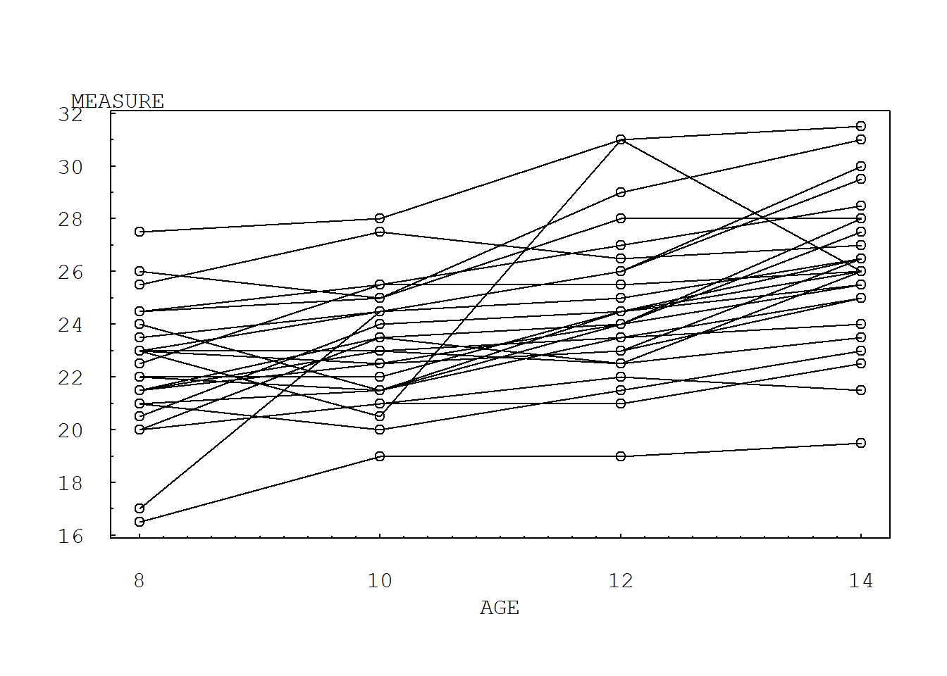
From Figure 5.1, we can see that the measurement length grows as each child ages, although it is difficult to detect differences between boys and girls. In Figure 5.1, we use open circular plotting symbols for girls and filled circular plotting symbols for boys. Figure 5.1 does show that the ninth boy has an unusual growth pattern; this pattern can also be seen in Table 5.1.
5.2.2 Summary statistics
summary(Dental[, c("MEASURE")]) Min. 1st Qu. Median Mean 3rd Qu. Max.
16.50 22.00 23.75 24.02 26.00 31.50 5.2.3 Trellis plot, unique in r
dent1 = groupedData(MEASURE ~ AGE | ID, data=Dental, outer=~SEX)
plot(dent1, layout = c(16,2))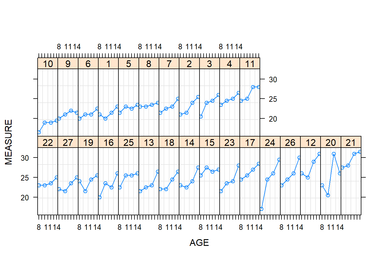
5.3 TABLE 5.2: Dental data growth-curve-model parameter estimates
5.3.1 TABLE 5.2: Error components model
dental1.lme<-lme(MEASURE~AGE*SEX, data=Dental, random=~1|ID)
summary(dental1.lme)
Linear mixed-effects model fit by REML
Data: Dental
AIC BIC logLik
445.7572 461.6236 -216.8786
Random effects:
Formula: ~1 | ID
(Intercept) Residual
StdDev: 1.816214 1.386382
Fixed effects: MEASURE ~ AGE * SEX
Value Std.Error DF t-value p-value
(Intercept) 16.340625 0.9813122 79 16.651810 0.0000
AGE 0.784375 0.0775011 79 10.120823 0.0000
SEX 1.032102 1.5374208 25 0.671321 0.5082
AGE:SEX -0.304830 0.1214209 79 -2.510520 0.0141
Correlation:
(Intr) AGE SEX
AGE -0.869
SEX -0.638 0.555
AGE:SEX 0.555 -0.638 -0.869
Standardized Within-Group Residuals:
Min Q1 Med Q3 Max
-3.59804400 -0.45461690 0.01578365 0.50244658 3.68620792
Number of Observations: 108
Number of Groups: 27 5.3.2 TABLE 5.2: Growth curve model
dental2.lme<-lme(MEASURE~AGE*SEX, data=Dental, random=~1+AGE|ID, correlation=corSymm(form=~1|ID),control= lmeControl(opt = "optim")) # I add the code "control= lmeControl(opt = "optim")" to fix converge problem
#corSymm gives a general correlation structure in lme
dental2.lme
Linear mixed-effects model fit by REML
Data: Dental
Log-restricted-likelihood: -213.0644
Fixed: MEASURE ~ AGE * SEX
(Intercept) AGE SEX AGE:SEX
15.9304961 0.8243798 1.4779148 -0.3483069
Random effects:
Formula: ~1 + AGE | ID
Structure: General positive-definite, Log-Cholesky parametrization
StdDev Corr
(Intercept) 1.73852535 (Intr)
AGE 0.07167425 -0.238
Residual 1.49360182
Correlation Structure: General
Formula: ~1 | ID
Parameter estimate(s):
Correlation:
1 2 3
2 0.015
3 0.172 0.017
4 -0.111 0.431 0.341
Number of Observations: 108
Number of Groups: 27 5.3.3 TABLE 5.2: Growth curve model - omitting 9th boy
Dental2<-subset(Dental, ID!=20)
dental3.lme<-update(dental2.lme, data=Dental2)
dental3.lme
Linear mixed-effects model fit by REML
Data: Dental2
Log-restricted-likelihood: -188.7711
Fixed: MEASURE ~ AGE * SEX
(Intercept) AGE SEX AGE:SEX
16.8586091 0.7699492 0.6119536 -0.2975491
Random effects:
Formula: ~1 + AGE | ID
Structure: General positive-definite, Log-Cholesky parametrization
StdDev Corr
(Intercept) 1.63375372 (Intr)
AGE 0.06425145 0.028
Residual 1.28363690
Correlation Structure: General
Formula: ~1 | ID
Parameter estimate(s):
Correlation:
1 2 3
2 -0.200
3 0.080 0.518
4 -0.511 0.169 0.562
Number of Observations: 104
Number of Groups: 26 Table 5.2 shows the parameter estimates for this model. Here, we see that the coefficient associated with linear growth is statistically significant, over all models. Moreover, the rate of increase for girls is lower than for boys. The estimated covariance between \(\alpha_{0i}\) and \(\alpha_{1i}\) (which is also the estimated covariance between \(\beta_{0i}\) and \(β_{1i}\) turns out to be negative. One interpretation of the negative covariance between initial status and growth rate is that subjects who start at a low level tend to grow more quickly than those who start at higher levels, and vice versa.
For comparison purposes, Table 5.2 shows the parameter estimates with the ninth boy deleted. The effects of this subject deletion on the parameter estimates are small. Table 5.2 also shows parameter estimates of the errorcomponents model. This model employs the same level-1 model but with level-2 models
\[\beta_{0i}=\beta_{00}+\beta_{01} \text{GENDER}_i + \alpha_{0i}\]
\[\beta_{1i}=\beta_{10}+\beta_{11} \text{GENDER}_i\] With parameter estimates calculated using the full data set, there again is little change in the parameter estimates. Because the results appear to be robust to both unusual subjects and model selection, we have greater confidence in our interpretations.